Python环境配置与数据处理

最新推荐文章于 2024-07-20 17:12:48 发布

啥也没学懂

最新推荐文章于 2024-07-20 17:12:48 发布

阅读量2.2k

点赞数 2

文章标签： python numpy 开发语言

本文链接：https://blog.csdn.net/qq_53916653/article/details/129445695

版权

一、环境配置

1.Anaconda安装与配置

在官网下载 Anaconda 的最新版本：https://www.anaconda.com/

创建虚拟环境

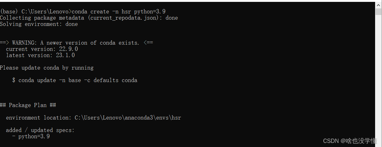
首先我们需要打开 Anaconda Prompt (在开始菜单中)

在默认路径下创建虚拟环境

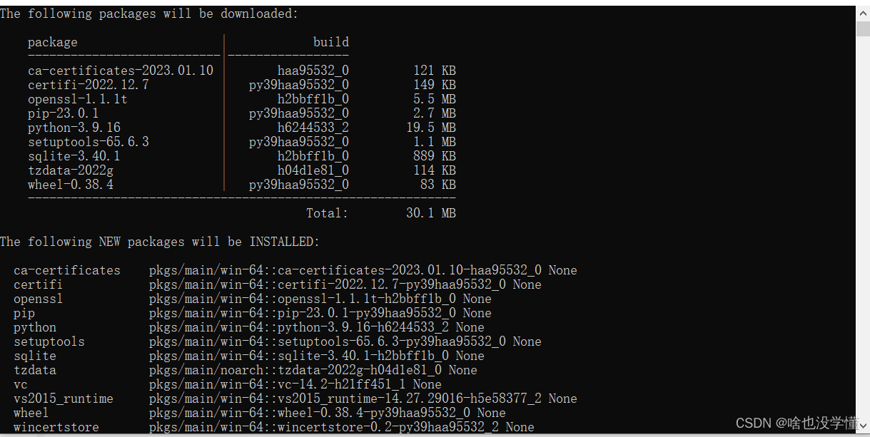
conda create -n hsr python=3.9 # 这里的默认 python 设置为 python 3.9

在这里插入图片描述

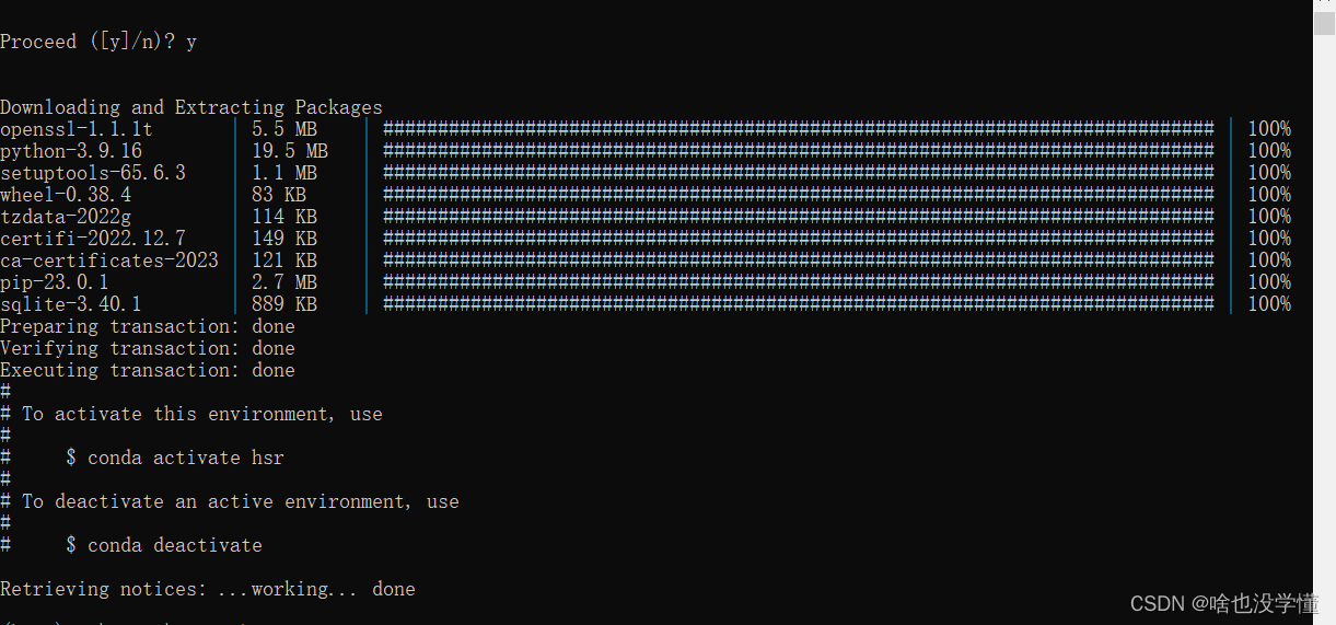
开启与切换虚拟环境

激活虚拟环境

activate hsr

我们可以使用如下命令切换虚拟环境：

conda activate hsr

在这里插入图片描述

删除虚拟环境

方法一：

首先退出环境

conda deactivate

查看虚拟环境列表，此时出现列表的同时还会显示其所在路径

conda env list

删除环境

conda env remove -n 要删除的虚拟环境名称
conda env remove -p 要删除的虚拟环境路径
# 删除命令后面可以加上 -all 删除掉所有配置环境

方法二：

首先退出环境

conda deactivate

删除环境

conda remove -n  需要删除的环境名 --all

2.安装 jupyter 和 numpy

安装jupyter命令：

conda install -n myconda jupyter notebook

安装numpy命令：

conda install -n myconda numpy

检验jupyter是否安装成功
在上述环境中输入命令打开jupyter

jupyter notebook

在这里插入图片描述

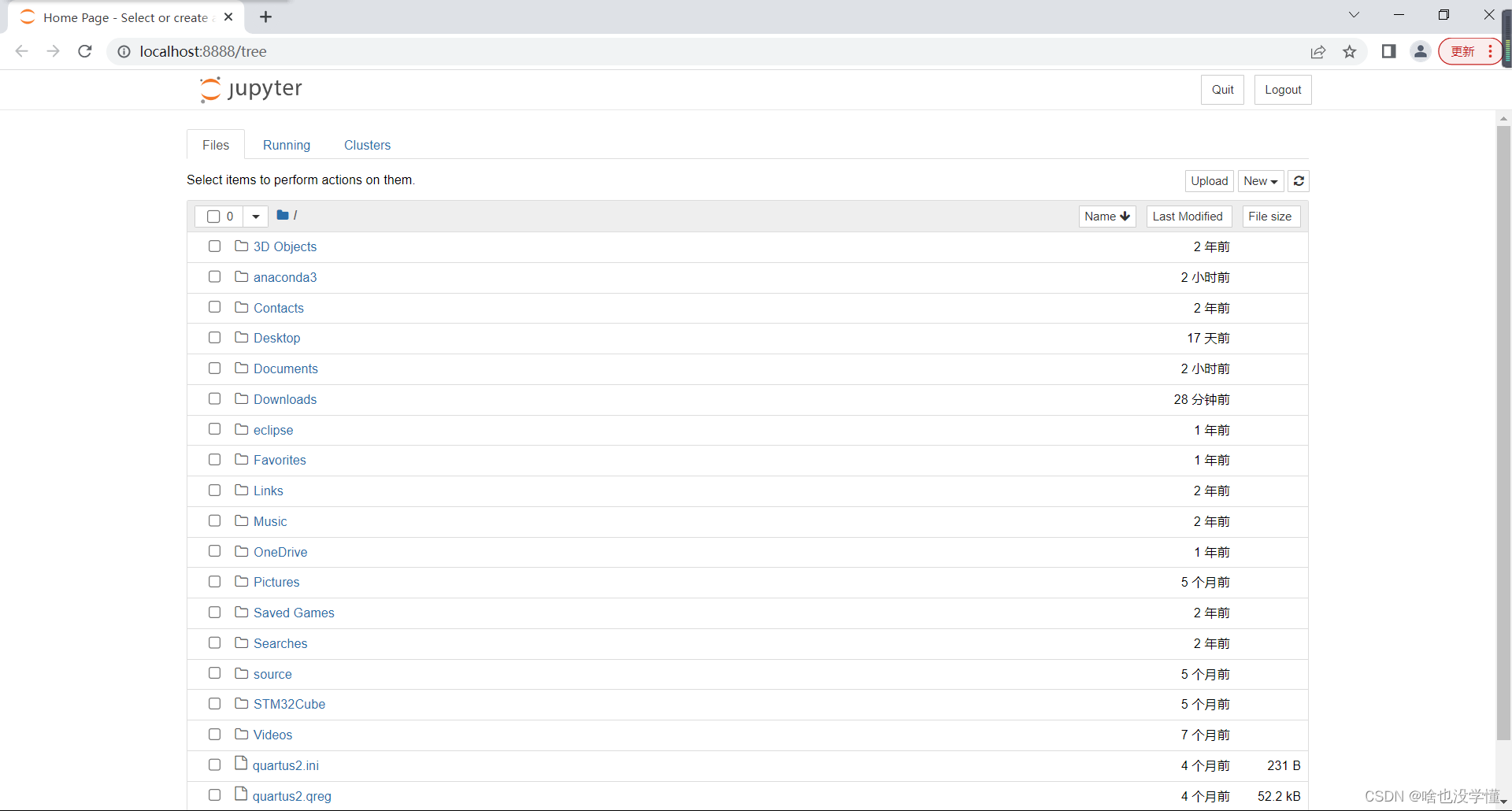
出现该页面说明jupyter安装成功，可以进行接下来的numpy的基础练习了。

二、numpy基础练习

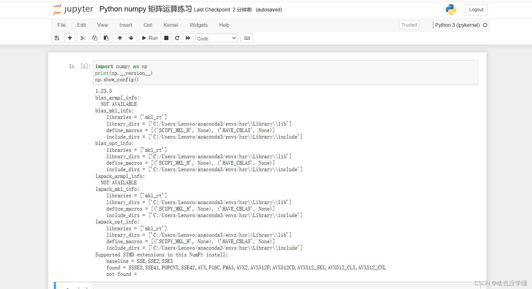
查看 numpy 版本和配置：

import numpy as np
print(np.__version__)
np.show_config()

在这里插入图片描述

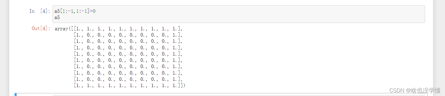
1.创建一个10*10的ndarray对象，且矩阵边界全为1，里面全为0

#创建一个10*10的ndarray对象，且矩阵边界全为1，里面全为0

import numpy as np
nd = np.zeros(shape = (10,10),dtype = np.int8)
nd[[0,9]] = 1

nd[:,[0,9]] = 1
nd

a5=np.ones((10,10))
a5

a5[1:-1,1:-1]=0
a5

在这里插入图片描述

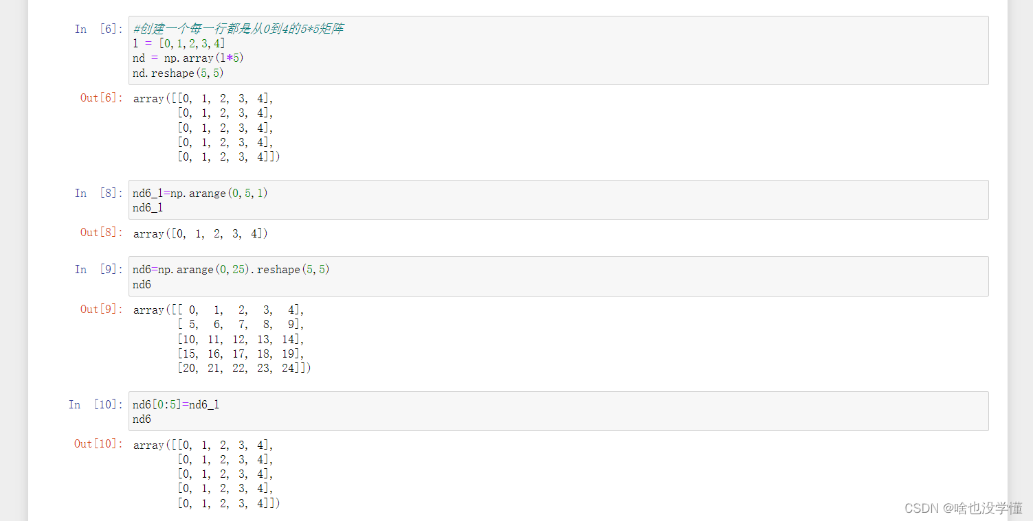
2.创建一个每一行都是从0到4的5*5矩阵

#创建一个每一行都是从0到4的5*5矩阵
l = [0,1,2,3,4]
nd = np.array(l*5)
nd.reshape(5,5)

nd6_l=np.arange(0,5,1)
nd6_l

nd6=np.arange(0,25).reshape(5,5)
nd6

nd6[0:5]=nd6_l
nd6

在这里插入图片描述

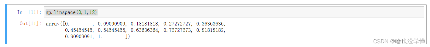
3.创建一个范围在(0,1)之间的长度为12的等差数列

np.linspace(0,1,12)

在这里插入图片描述

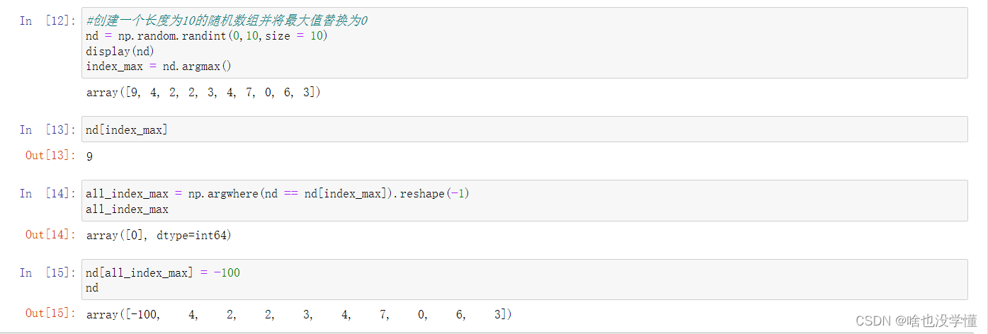
4.创建一个长度为10的随机数组并将最大值替换为0

#创建一个长度为10的随机数组并将最大值替换为0
nd = np.random.randint(0,10,size = 10)
display(nd)
index_max = nd.argmax()

nd[index_max]

all_index_max = np.argwhere(nd == nd[index_max]).reshape(-1)
all_index_max

nd[all_index_max] = -100
nd

在这里插入图片描述

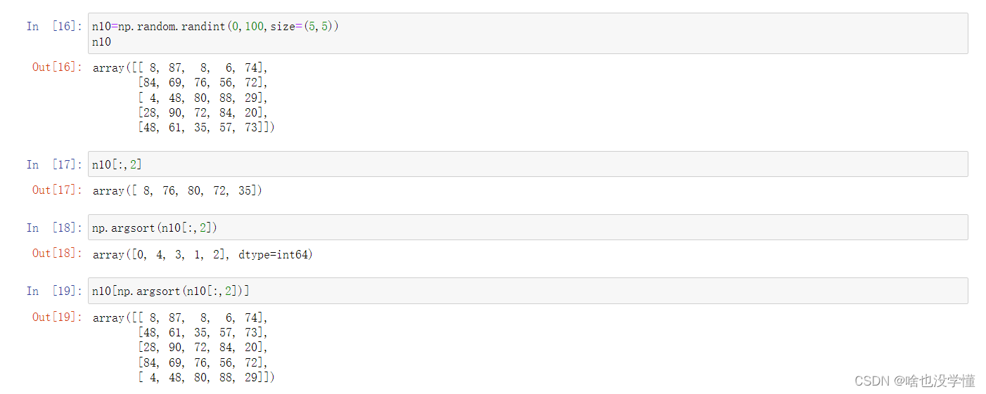
5.如何根据第3列来对一个5*5矩阵排序？

n10=np.random.randint(0,100,size=(5,5))
n10
n10[:,2]
np.argsort(n10[:,2])
n10[np.argsort(n10[:,2])]

在这里插入图片描述

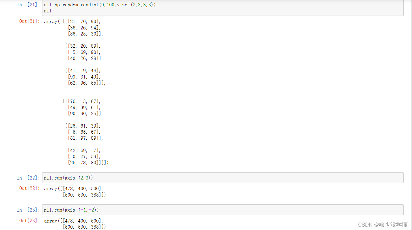
6.给定一个4维矩阵，如何得到最后两维的和？

nll=np.random.randint(0,100,size=(2,3,3,3))
nll

nll.sum(axis=(2,3))

nll.sum(axis=(-1,-2))

在这里插入图片描述

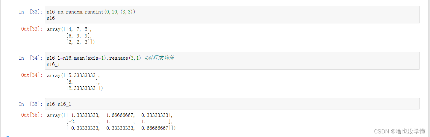
7.矩阵的每一行的元素都减去该行的平均值

n16=np.random.randint(0,10,(3,3))
n16

n16_1=n16.mean(axis=1).reshape(3,1) #对行求均值
n16_1

n16-n16_1

在这里插入图片描述

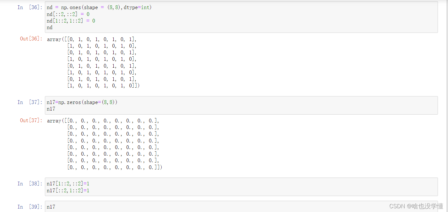
8.打印出以下函数（要求使用np.zeros创建8*8的矩阵）：

[[0 1 0 1 0 1 0 1]
[1 0 1 0 1 0 1 0]
[0 1 0 1 0 1 0 1]
[1 0 1 0 1 0 1 0]
[0 1 0 1 0 1 0 1]
[1 0 1 0 1 0 1 0]
[0 1 0 1 0 1 0 1]
[1 0 1 0 1 0 1 0]]

nd = np.ones(shape = (8,8),dtype=int)
nd[::2,::2] = 0
nd[1::2,1::2] = 0
nd

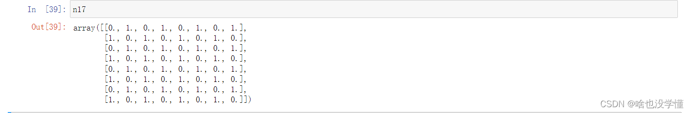
n17=np.zeros(shape=(8,8))
n17

n17[1::2,::2]=1
n17[::2,1::2]=1
n17

在这里插入图片描述

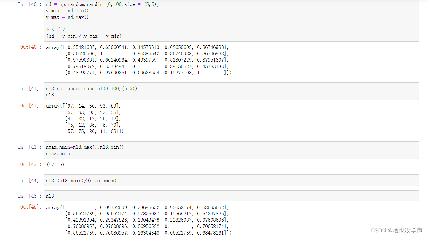
9.正则化一个5*5随机矩阵

【正则的概念：假设a是矩阵中的一个元素，max/min分别是矩阵元素的最大最小值，则正则化后a = (a - min)/(max - min)】

nd = np.random.randint(0,100,size = (5,5))
v_min = nd.min()
v_max = nd.max()

# 0 ~ 1
(nd - v_min)/(v_max - v_min)

n18=np.random.randint(0,100,(5,5))
n18

nmax,nmin=n18.max(),n18.min()
nmax,nmin

n18=(n18-nmin)/(nmax-nmin)

n18

在这里插入图片描述

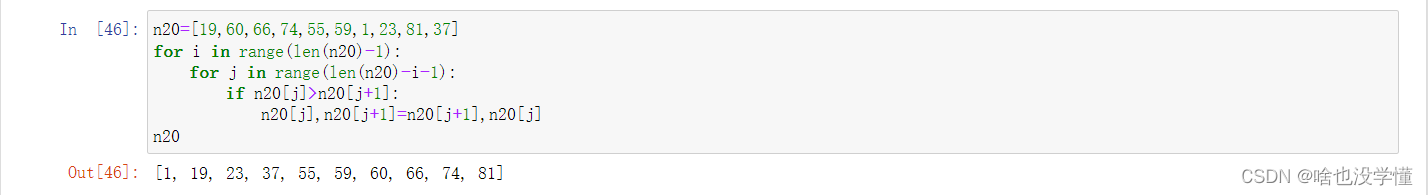
10.实现冒泡排序法

n20=[19,60,66,74,55,59,1,23,81,37]
for i in range(len(n20)-1):
    for j in range(len(n20)-i-1):
        if n20[j]>n20[j+1]:
            n20[j],n20[j+1]=n20[j+1],n20[j]
n20

在这里插入图片描述

三、Python基础例题

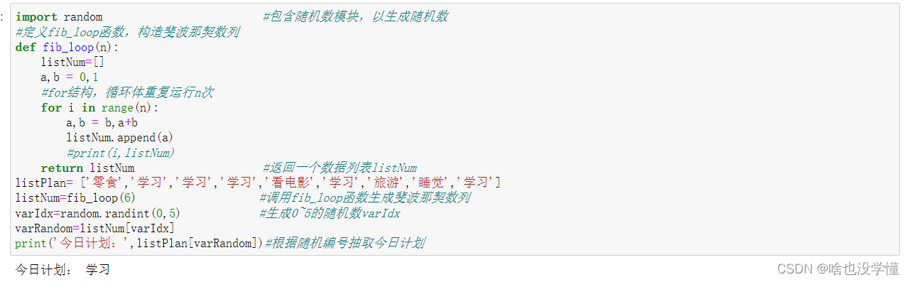
1.Python语言综合示例——天天学习，天天向上。

import random                         #包含随机数模块，以生成随机数
#定义fib_loop函数，构造斐波那契数列
def fib_loop(n):
    listNum=[]
    a,b = 0,1
    #for结构，循环体重复运行n次
    for i in range(n):
        a,b = b,a+b
        listNum.append(a)
        #print(i,listNum)
    return listNum                    #返回一个数据列表listNum
listPlan= ['零食','学习','学习','学习','看电影','学习','旅游','睡觉','学习']
listNum=fib_loop(6)                   #调用fib_loop函数生成斐波那契数列
varIdx=random.randint(0,5)            #生成0~5的随机数varIdx
varRandom=listNum[varIdx]
print('今日计划：',listPlan[varRandom])#根据随机编号抽取今日计划

在这里插入图片描述

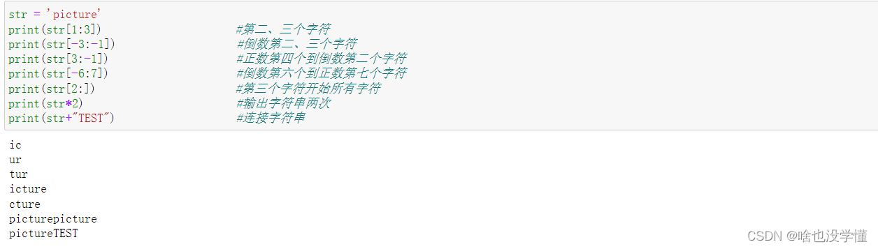
2.字符串的访问

str = 'picture'
print(str[1:3])                     #第二、三个字符
print(str[-3:-1])                   #倒数第二、三个字符
print(str[3:-1])                    #正数第四个到倒数第二个字符
print(str[-6:7])                    #倒数第六个到正数第七个字符
print(str[2:])                      #第三个字符开始所有字符
print(str*2)                        #输出字符串两次
print(str+"TEST")                   #连接字符串

在这里插入图片描述

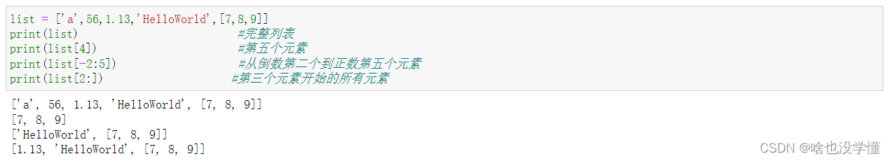
3.列表的访问

list = ['a',56,1.13,'HelloWorld',[7,8,9]]
print(list)                         #完整列表
print(list[4])                      #第五个元素
print(list[-2:5])                   #从倒数第二个到正数第五个元素
print(list[2:])                    #第三个元素开始的所有元素

在这里插入图片描述

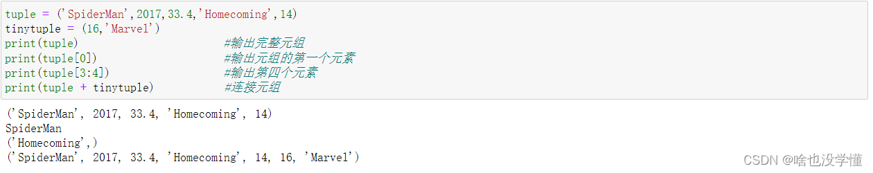
4.元组的访问

tuple = ('SpiderMan',2017,33.4,'Homecoming',14)
tinytuple = (16,'Marvel')
print(tuple)                       #输出完整元组
print(tuple[0])                    #输出元组的第一个元素
print(tuple[3:4])                  #输出第四个元素
print(tuple + tinytuple)           #连接元组

在这里插入图片描述

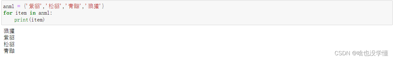
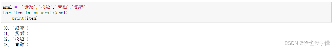
5.有一个集合anml，其内容为{‘紫貂’，‘松貂’，‘青鼬’，‘狼獾’}，对anml集合进行遍历。

方法一：

anml = {'紫貂','松貂','青鼬','狼獾'}
for item in anml:
    print(item)

在这里插入图片描述

方法二：

anml = {'紫貂','松貂','青鼬','狼獾'}
for item in enumerate(anml):
    print(item)

在这里插入图片描述

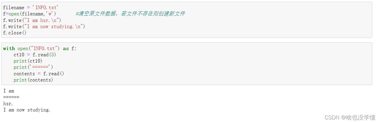
6.写入文件并打开

打开文件并写入数据

filename = 'INFO.txt'
f=open(filename,'w')       #清空原文件数据，若文件不存在则创建新文件
f.write("I am hsr.\n")
f.write("I am now studying.\n")
f.close()

read()函数读取文件

with open("INFO.txt") as f:
    ct10 = f.read(5)
    print(ct10)
    print('======')
    contents = f.read()
    print(contents)

在这里插入图片描述

四、Python综合练习

1.NumPy

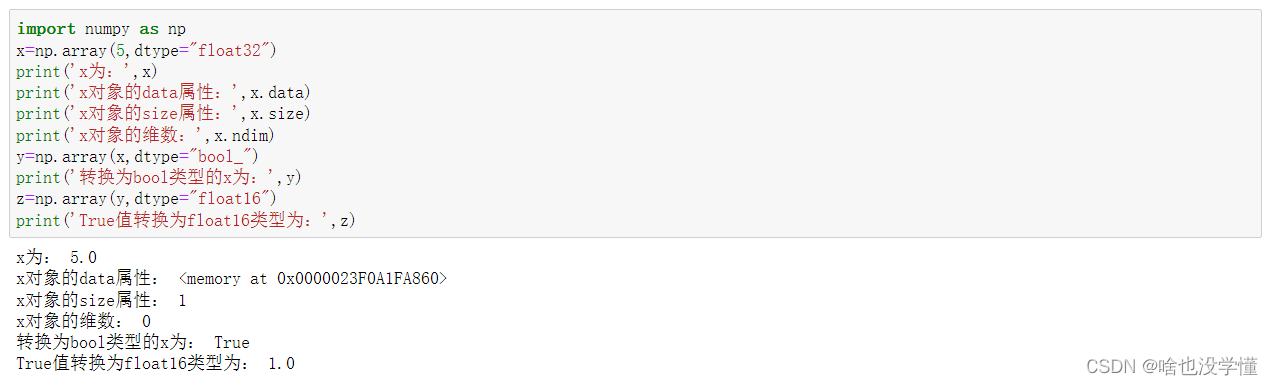
使用dtype对象设置数据类型

import numpy as np
x=np.array(5,dtype="float32")
print('x为：',x)
print('x对象的data属性：',x.data)
print('x对象的size属性：',x.size)
print('x对象的维数：',x.ndim)
y=np.array(x,dtype="bool_")
print('转换为bool类型的x为：',y)
z=np.array(y,dtype="float16")
print('True值转换为float16类型为：',z)

在这里插入图片描述

简单条件运算

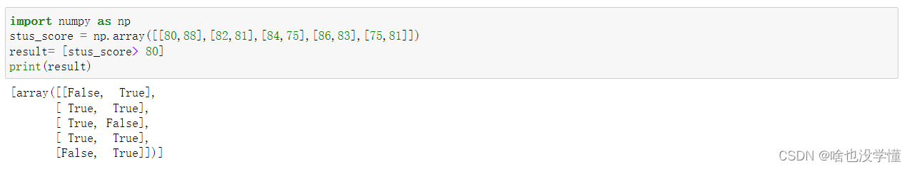
import numpy as np
stus_score = np.array([[80,88],[82,81],[84,75],[86,83],[75,81]])
result= [stus_score> 80]
print(result)

在这里插入图片描述

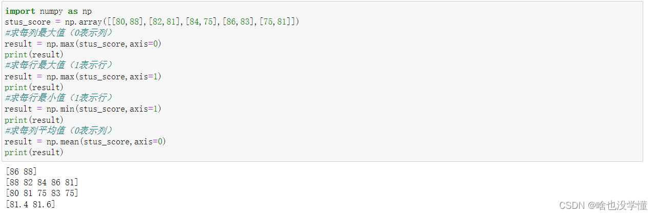
ndarray的统计计算。

import numpy as np
stus_score = np.array([[80,88],[82,81],[84,75],[86,83],[75,81]])
#求每列最大值（0表示列）
result = np.max(stus_score,axis=0)
print(result)
#求每行最大值（1表示行）
result = np.max(stus_score,axis=1)
print(result)
#求每行最小值（1表示行）
result = np.min(stus_score,axis=1)
print(result)
#求每列平均值（0表示列）
result = np.mean(stus_score,axis=0)
print(result)

在这里插入图片描述

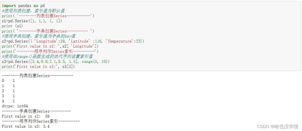
2.Pandas

为一个地理位置数据创建Series对象。

import pandas as pd
#使用列表创建，索引值为默认值
print( '--------列表创建Series-----------')
s1=pd.Series([1, 1,1, 1, 1])
print (s1)
print( '--------字典创建Series---------- ')
#使用字典创建，索引值为字典的key值
s2=pd.Series({ 'Longitude':39, 'Latitude' :116, 'Temperature':23})
print('First value in s2: ',s2[ 'Longitude'])
print('--------用序列作Series索引----------')
#使用由range()函数生成的迭代序列设置索引值
s3=pd.Series([3.4,0.8,2.1,0.3, 1.5], range(5, 10))
print('First value in s3:', s3[5])

在这里插入图片描述

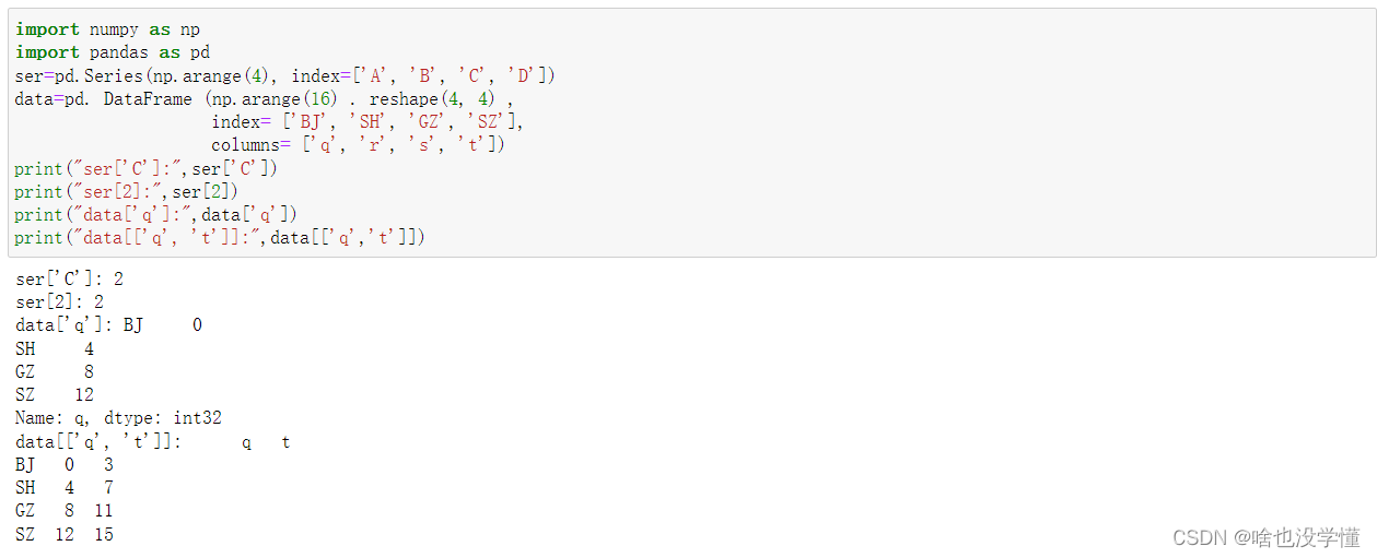
对Series和DataFrame进行索引

import numpy as np
import pandas as pd
ser=pd.Series(np.arange(4), index=['A', 'B', 'C', 'D'])
data=pd. DataFrame (np.arange(16) . reshape(4, 4) ,
                    index= ['BJ', 'SH', 'GZ', 'SZ'],
                    columns= ['q', 'r', 's', 't'])
print("ser['C']:",ser['C'])
print("ser[2]:",ser[2])
print("data['q']:",data['q'])
print("data[['q', 't']]:",data[['q','t']])

在这里插入图片描述

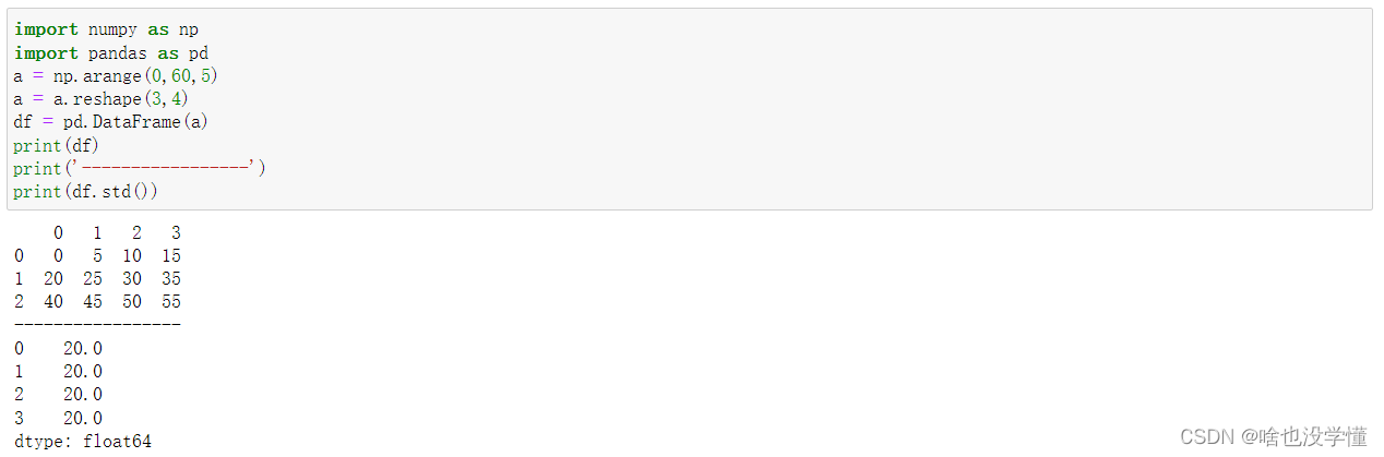
使用Pandas模块求方差。

import numpy as np
import pandas as pd
a = np.arange(0,60,5)
a = a.reshape(3,4)
df = pd.DataFrame(a)
print(df)
print('-----------------')
print(df.std())

在这里插入图片描述

3.Matplotlib

引入库：

import numpy as np
import matplotlib
import matplotlib.mlab as mlab
import matplotlib.pyplot as plt

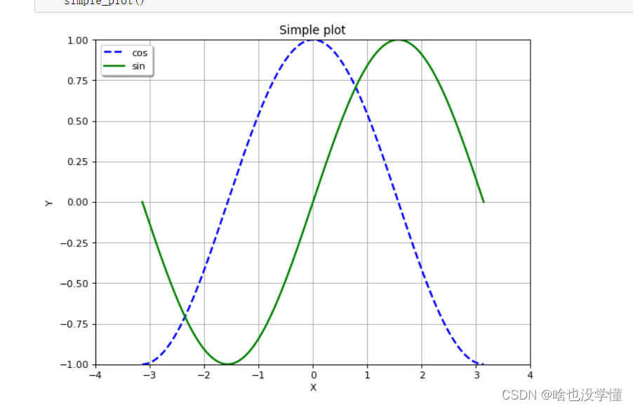
正弦函数余弦函数

def simple_plot():
    # 生成测试数据
    x = np.linspace(-np.pi, np.pi, 256, endpoint=True)
    y_cos, y_sin = np.cos(x), np.sin(x)
 
    # 生成画布，并设定标题
    # 画布大小，dpi＝清晰度
    plt.figure(figsize=(8, 6), dpi=80)
    plt.title("Simple plot")
    plt.grid(True)  # 带网格
 
    # 设置X轴
    plt.xlabel("X")
    plt.xlim(-4.0, 4.0)
    plt.xticks(np.linspace(-4, 4, 9, endpoint=True))
 
    # 设置Y轴
    plt.ylabel("Y")
    plt.ylim(-1.0, 1.0)
    plt.yticks(np.linspace(-1, 1, 9, endpoint=True))
 
    # 画两条曲线
    plt.plot(x, y_cos, "b--", linewidth=2.0, label="cos")
    plt.plot(x, y_sin, "g-", linewidth=2.0, label="sin")
 
    # 设置图例位置,loc可以为[upper, lower, left, right, center]
    plt.legend(loc="upper left",shadow=True) 
 
    # 图形显示
    plt.show()
    return
if __name__ == "__main__":
# 运行
    simple_plot()

在这里插入图片描述

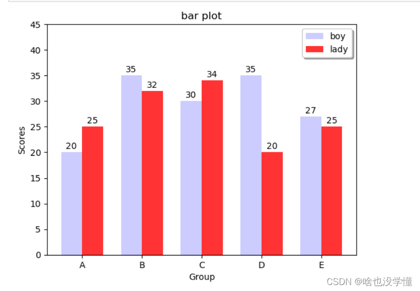
柱状图

# 柱状图
def bar_plot():
    """
    bar plot
    """
    # 生成测试数据
    means_men = (20, 35, 30, 35, 27)
    means_women = (25, 32, 34, 20, 25)
 
    # 设置标题
    plt.title("bar plot")
 
    # 设置相关参数
    index = np.arange(len(means_men))
    bar_width = 0.35
 
    # 画柱状图
    plt.bar(index, means_men, width=bar_width, alpha=0.2, color="b", label="boy")
    plt.bar(index+bar_width, means_women, width=bar_width, alpha=0.8, color="r", label="lady")
    plt.legend(loc="upper right",shadow=True)
 
    # 设置柱状图标示
    for x, y in zip(index, means_men):
        plt.text(x, y+0.3, y, ha="center", va="bottom")
    for x, y in zip(index, means_women):
        plt.text(x+bar_width, y+0.3, y, ha="center", va="bottom")
 
    # 设置刻度范围/坐标轴名称等
    plt.ylim(0, 45)
    plt.xlabel("Group")
    plt.ylabel("Scores")
    plt.xticks(index+(bar_width/2), ("A", "B", "C", "D", "E"))
 
    # 图形显示
    plt.show()
    return
 
# 横向柱状图
def barh_plot():
    """
    barh plot
    """
    # 生成测试数据
    means_men = (20, 35, 30, 35, 27)
    means_women = (25, 32, 34, 20, 25)
 
    # 设置标题
    plt.title("barh plot")
 
    # 设置相关参数
    index = np.arange(len(means_men))
    bar_height = 0.35
 
    # 画柱状图(水平方向)
    plt.barh(index, means_men, height=bar_height, alpha=0.2, color="b", label="Men")
    plt.barh(index+bar_height, means_women, height=bar_height, alpha=0.8, color="r", label="Women")
    plt.legend(loc="upper right", shadow=True)
 
    # 设置柱状图标示
    for x, y in zip(index, means_men):
        plt.text(y+0.3, x, y, ha="left", va="center")
    for x, y in zip(index, means_women):
        plt.text(y+0.3, x+bar_height, y, ha="left", va="center")
 
    # 设置刻度范围/坐标轴名称等
    plt.xlim(0, 45)
    plt.xlabel("Scores")
    plt.ylabel("Group")
    plt.yticks(index+(bar_height/2), ("A", "B", "C", "D", "E"))
 
    # 图形显示
    plt.show()
    return
if __name__ == "__main__":
# 运行
    bar_plot()
    barh_plot()

在这里插入图片描述

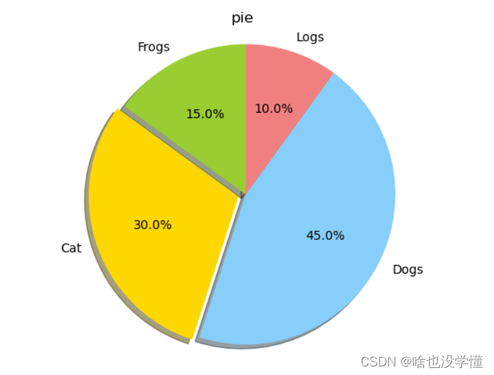
饼状图

# 饼图
def pie_plot():
    """
    pie plot
    """
    # 生成测试数据
    sizes = [15, 30, 45, 10]
    labels = ["Frogs", "Cat", "Dogs", "Logs"]
    colors = ["yellowgreen", "gold", "lightskyblue", "lightcoral"]
 
    # 设置标题
    plt.title("pie")
 
    # 设置突出参数
    explode = [0, 0.05, 0, 0]
 
    # 画饼状图
    patches, l_text, p_text = plt.pie(sizes, explode=explode, labels=labels, colors=colors, autopct="%1.1f%%", shadow=True, startangle=90)
 
    plt.axis("equal")
 
    # 图形显示
    plt.show()
    return
if __name__ == "__main__":
# 运行
    pie_plot()

在这里插入图片描述

五、图灵测试

测试内容

如果一个人(代号C)使用测试对象皆理解的语言去询问两个他不能看见的对象任意一串问题。对象为：一个是正常思维的人(代号B)、一个是机器(代号A)。如果经过若干询问以后，C 不能得出实质的区别来分辨 A 与 B 的不同，则此机器 A 通过图灵测试

完成图灵测试涉及的技术课题：

根据人们的大体判断，达成能够通过图灵测试的技术涉及以下课题：

1.自然语言处理
2.知识表示
3.自动推理
4.机器学习

但是为了通过完全图灵测试，还需要另外两项额外技术课题：

1.计算机视觉
2.机器人学

图灵测试的变种：

许多其他版本的图灵测试，包括上文所阐述的，已经经过多年的酝酿

反向图灵测试和验证码：

验证码(CAPTCHA)是一种反向图灵测试。在网站上执行一些操作前，用户被给予一个扭曲的图形，并要求用户输入图中的字母或数字。这是为了防止网站被自动化系统滥用。理由是能够精细地阅读和准确地重现扭曲的形象的系统并不存在(或不提供给普通用户)，所以能够做到这一点的任何系统可能是个人类

可以破解验证码的软件正在积极开发，软件拥有一个有一定准确性的验证码分析模式生成引擎。而在破解验证码软件被积极开发的同时，另一种通过反向图灵测试的准则也被提出来。其认为即使破解验证码软件被成功研发，也只是具有智能的人类透过编程对验证码所作出的破解手段而已，并非真正通过反向图灵测试或图灵测试。而如果一台机器能够规划出如同验证码一类的防止自动化系统的规避程序，此台机器才算是真正通过了反向图灵测试

完全图灵测试：

普通的图灵测试一般避免审问者与被测试计算机发生物理上的互动，因为物理上模拟人(比如像模拟人的外表)并不是人工智能的研究范畴。然而一些人工智能可能涉及一些人机在物理上的交互，所以人们又拓展出了“完全图灵测试”。在完全图灵测试中，可以包含必要的人机在物理层面上的交互。但是为了通过完全图灵测试，还需要在普通图灵测试之外另外两项额外技术课题。询问者还可以测试受试者的感知能力(需要电脑视觉)，和受试者操纵物体的能力(需要机器人学)