


pandas的简单使用(数据统计)
统计
如果DataFrame里全是数值,那么汇总类的统计,就可以不加列名。
比如求和
- df.sum(axis=1) 是求每一行的和。等价于 df.apply(np.sum,axis=1)
- df.sum(axis=0) 是求每一列的和。等价于 df.apply(np.sum,axis=0)
均值最值方差那些也是一样的。
汇总类统计(针对数值型)
# 统计每一列的个数
df.count()

# 统计非空值的个数(一般搭配列使用)
# 下面三行结果一样
df['weight'].value_counts()
df.value_counts('weight')
df.groupby('weight').size()

# 下面三行结果一样(但效果上groupby更好)
df[['age','weight']].value_counts()
df.value_counts(['age','weight'])
df.groupby(['age','weight']).size()


# 下面这些统计方法,一般搭配列使用,若不加大都会有警告
# 不加列df.sum(), 多个列df[['列1','列2']].sum()

# 计算累加
df['weigh'].sum()

# 统计均值
df['weigh'].mean()

# 统计中位数
df['weigh'].median()

# 统计最大值
df['weigh'].max()

# 统计最小值
df['weigh'].min()

# 统计方差
df['weigh'].var()

# 统计标椎差
df['weigh'].std()


# 对特定几列的数据进行统计分析
df.agg(
    {
        "Age": ["min", "max", "mean"],
        "weigh": ["min", "max", "mean"]
    }
)
>>> 输出
       Age    weigh
min     12    32.00
max     80   212.32
mean 29.69    52.20
描述性统计(针对数值型)
描述性统计只针对列数据是int型的。它能看出这一列中数据的分布情况
# 统计个数,计算均值,标椎差,最小值,一二三分位数,最大值(count   mean   std   min   25%   50%    75%    max)
a = data.describe()

# 加参数形式(参数过多,加个转置方便看)
aa = data.describe([0.01,0.1,0.25,0.5,0.75,0.9,0.99]).T
输出aa,,,
'''
# 描述性统计
# 列表里的数值与分位数有关,但不是分位数
# 分位数(Quantile),亦称分位点,是指将一个随机变量的概率分布范围分为几个等份的数值点,常用的有中位数(即二分位数)、四分位数、百分位数等。
# 四分位数(Quartile)也称四分位点,是指在统计学中把所有数值由小到大排列并分成四等份,处于三个分割点位置的数值。

打印结果:

                                         count         mean           std  min    1%        10%          25%          50%          75%           90%           99%        max
SeriousDlqin2yrs                      149391.0     0.066999      0.250021  0.0   0.0   0.000000     0.000000     0.000000     0.000000      0.000000      1.000000        1.0
RevolvingUtilizationOfUnsecuredLines  149391.0     6.071087    250.263672  0.0   0.0   0.003199     0.030132     0.154235     0.556494      0.978007      1.093922    50708.0
age                                   149391.0    52.306237     14.725962  0.0  24.0  33.000000    41.000000    52.000000    63.000000     72.000000     87.000000      109.0
NumberOfTime30-59DaysPastDueNotWorse  149391.0     0.393886      3.852953  0.0   0.0   0.000000     0.000000     0.000000     0.000000      1.000000      4.000000       98.0
DebtRatio                             149391.0   354.436740   2041.843455  0.0   0.0   0.034991     0.177441     0.368234     0.875279   1275.000000   4985.100000   329664.0
MonthlyIncome                         149391.0  5426.886926  13245.623932  0.0   0.0   0.180000  1800.000000  4425.000000  7416.000000  10800.000000  23205.000000  3008750.0
NumberOfOpenCreditLinesAndLoans       149391.0     8.480892      5.136515  0.0   0.0   3.000000     5.000000     8.000000    11.000000     15.000000     24.000000       58.0
NumberOfTimes90DaysLate               149391.0     0.238120      3.826165  0.0   0.0   0.000000     0.000000     0.000000     0.000000      0.000000      3.000000       98.0
NumberRealEstateLoansOrLines          149391.0     1.022391      1.130196  0.0   0.0   0.000000     0.000000     1.000000     2.000000      2.000000      4.000000       54.0
NumberOfTime60-89DaysPastDueNotWorse  149391.0     0.212503      3.810523  0.0   0.0   0.000000     0.000000     0.000000     0.000000      0.000000      2.000000       98.0
NumberOfDependents                    149391.0     0.759863      1.101749  0.0   0.0   0.000000     0.000000     0.000000     1.000000      2.000000      4.000000       20.0

月收入(MonthlyIncome)这一行,最小值是0,最大值是3008750。收入在0.18以下的人有10%,在1800以下的人有25%,中位数是4425,月收入超过23205的只有1%
过去两年内出现35-59天逾期但是没有发展得更坏的次数(NumberOfTime30-59DaysPastDueNotWorse),说明有75%的数都是0。实际上0有125453个,而数据才有149391行
'''
相关系数和协方差(针对数值型)
# 协方差矩阵(输出列之间 两两对应的协方差)
df.cov()


# 相关系数矩阵(输出列之间 两两对应的相关系数)
df.corr()


# 单独查看两个列之间
df['气候'].cov(df['最高温'])
df['气候'].corr(df['最高温'])


# 添加点运算的
df['气候'].cov(df['最高温']-df['最低温'])
df['气候'].corr(df['最高温']-df['最低温'])
不挑类型的统计
# 统计每一列的个数
df.count()


# 统计值的个数(一般搭配列使用)
# 不加列df.value_counts(), 多个列df[['列1','列2']].value_counts()
df['班级'].value_counts()


# 找出这一列中的唯一值,类型是<class 'numpy.ndarray'>  类似于 set(df['班级'])
df['班级'].unique()
统计相关的筛选
df = pd.DataFrame({
   "A": [4, 23, 22, 54, 16],
   "B": [1, 12, 65, 11, 27],
   "C": [22, 11, 18, 12, 25]
})
idxmin() dxmax()
idxmin()和idxmax()方法,用来查找表格当中最大/最小值的位置,返回的是值的索引
用在DataFrame
print(df.idxmax())
'''
A    3
B    2
C    4
dtype: int64
'''
# axis值默认为0。当值为1时,统计结果如下
print(df.idxmax(axis=1))
'''
0    C
1    A
2    B
3    A
4    B
dtype: object
'''
用在Series
print(df['A'].idxmin())  # 0
print(df['A'].idxmax())  # 3
nsmallest() nlargest()
nsmallest 以及 nlargest 方法是用来找到数据集当中最小、最大的若干数据。(相当于排序后在截取)
print(df.nsmallest(2, "A"))
'''
    A   B   C
0   4   1  22
4  16  27  25
'''
print(df.nlargest(2, "A"))
'''
    A   B   C
3  54  11  12
1  23  12  11
'''
groupby分组统计
对于要用到groupby的情况,我更习惯于写SQL
from pandasql import sqldf
print(sqldf(‘select * from df’, globals()))
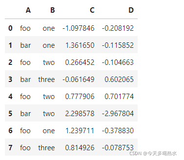
import pandas as pd
import numpy as np
df = pd.DataFrame({'A': ['foo', 'bar', 'foo', 'bar', 'foo', 'bar', 'foo', 'foo'],
                   'B': ['one', 'one', 'two', 'three', 'two', 'two', 'one', 'three'],
                   'C': np.random.randn(8),
                   'D': np.random.randn(8)})
单个列groupby,查询所有数据列的统计
print(df.groupby('A').sum())
'''
	     C	       D
A
bar	 3.598579	-2.481592
foo	 2.001150	-0.068664
'''
多个列groupby,查询所有数据列的统计
print(df.groupby(['A','B']).mean())
'''
		        C	        D
A	 B
bar	 one	 1.361650	-0.115852
     three	-0.061649	 0.602065
     two	 2.298578	-2.967804
foo	 one	 0.070933	-0.293511
     three   0.814926	-0.078753
     two	 0.522179	 0.298556
'''
添加参数:as_index=False
print(df.groupby(['A','B'], as_index=False).mean())
'''
	A	B	C	D
0	bar	one	    1.361650	-0.115852
1	bar	three  -0.061649	 0.602065
2	bar	two	    2.298578	-2.967804
3	foo	one	    0.070933	-0.293511
4	foo	three	0.814926	-0.078753
5	foo	two	    0.522179	 0.298556
'''
同时查看多种数据统计
print(df.groupby('A').agg([np.sum, np.mean, np.std, np.max]))
'''
	C	                                D
    sum         mean        std	        sum         mean	    std
A
bar	3.598579	1.199526	1.188437	-2.481592	-0.827197	1.888253
foo	2.001150	0.400230	0.905741	-0.068664	-0.013733	0.417000
'''
查看单列的结果数据统计
# 方法一
print(df.groupby('A')['C'].agg([np.sum, np.mean, np.std, np.max]))

# 方法二
print(df.groupby('A').agg([np.sum, np.mean, np.std, np.max])['C'])

'''
	sum	        mean	    std
A
bar	3.598579	1.199526	1.188437
foo	2.001150	0.400230	0.905741
'''
不同列使用不同的聚合函数
print(df.groupby('A').agg({"C":np.sum, "D":np.mean}))
'''
	C	        D
A
bar	3.598579	-0.827197
foo	2.001150	-0.013733
'''
遍历groupby的结果理解执行流程
遍历单个列聚合的分组
g = df.groupby('A')
print(g)
'''
<pandas.core.groupby.DataFrameGroupBy object at 0x000001EF8C3C2E80>
'''
遍历g这个对象,发现它依据A列的值,将原数据分成了两组
for name,group in g:
    print(name)
    print(group)
    print('-'*50)
'''
bar
     A      B         C         D
1  bar    one  1.361650 -0.115852
3  bar  three -0.061649  0.602065
5  bar    two  2.298578 -2.967804
--------------------------------------------------
foo
     A      B         C         D
0  foo    one -1.097846 -0.208192
2  foo    two  0.266452 -0.104663
4  foo    two  0.777906  0.701774
6  foo    one  1.239711 -0.378830
7  foo  three  0.814926 -0.078753
--------------------------------------------------
'''
可以获取单个分组的数据
g.get_group('bar')
'''
	A	B	C	D
1	bar	one	    1.361650	-0.115852
3	bar	three  -0.061649	 0.602065
5	bar	two	    2.298578	-2.967804
'''
遍历多个列聚合的分组
g = df.groupby(['A', 'B'])
for name,group in g:
    print(name)
    print(group)
    print('-'*50)

# 可以看到,name是一个2个元素的tuple,代表不同的列
'''
('bar', 'one')
     A    B        C         D
1  bar  one  1.36165 -0.115852
--------------------------------------------------
('bar', 'three')
     A      B         C         D
3  bar  three -0.061649  0.602065
--------------------------------------------------
('bar', 'two')
     A    B         C         D
5  bar  two  2.298578 -2.967804
--------------------------------------------------
('foo', 'one')
     A    B         C         D
0  foo  one -1.097846 -0.208192
6  foo  one  1.239711 -0.378830
--------------------------------------------------
('foo', 'three')
     A      B         C         D
7  foo  three  0.814926 -0.078753
--------------------------------------------------
('foo', 'two')
     A    B         C         D
2  foo  two  0.266452 -0.104663
4  foo  two  0.777906  0.701774
--------------------------------------------------
'''
g.get_group(('foo', 'one'))
'''
	A	B	C	D
0	foo	one	-1.097846	-0.208192
6	foo	one	1.239711	-0.378830
'''
g = df.groupby(['A', 'B'])
print(g['C'])
for name, group in g['C']:
    print(name)
    print(group)
    print(type(group))
    print('-'*50)
groupby的大体执行流程是
首先按照key进行分组,就可以得到每个group的名称以及group本身
而那些统计函数,都是在group上进行的
待计算完成之后,pandas会将key和统计结果拼接起来,得到一个结果的DataFrame
groupby实战样例
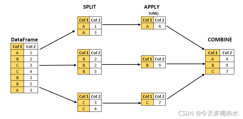
补充个知识点:Pandas的GroupBy遵从split、apply、combine模式。(DataFrame.groupby(‘Col1’).sum())
进入正题
import pandas as pd
import numpy as np

# df 一共有存放有366条数据,详细记录了2020年每一天的天气情况
df = pd.read_csv('F:\\Temp\\datas\\Tianqi_2020.csv')

# 添加一个月份列。时间是2020-10-10形式的
df['月份'] = df['时间'].str[:7]


# 查看每个月的最高温(1个月有30天,所以要在30个值中找出最大的) data1与data2相同
data1 = df.groupby('月份')['最高温'].max()
data2 = df.groupby('月份').max()['最高温']


# 查看每个月的最高温度、最低温度、平均空气质量指数
group_data = df.groupby('月份').agg({"最高温":np.max, "最低温":np.min, "空气指数":np.mean})


# 查看每个月温度最高的2天数据
def getWenduTopN(df, topn):
    # 这里的df,是每个月份分组group的df
    return df.sort_values(by="bWendu", ascending=False)[["月份", "最高温"]][:topn]
data = df.groupby("month").apply(getWenduTopN, topn=2)


# 画图
import matplotlib.pyplot as plt
plt.plot(data1)
plt.plot(group_data )
plt.show()


 1714
1714

 被折叠的 条评论
为什么被折叠?
被折叠的 条评论
为什么被折叠?
 到【灌水乐园】发言


