


原文链接:JoshiShamika/Deep-learning-for-Modulation-Recognition-on-RML2016.10a_dict-dataset (github.cs我对原文代码的修改:
import pickle
import matplotlib.pyplot as plt
import numpy as np
import pandas as pd

with open("2016/RML2016.10a_dict.pkl", 'rb') as file:
    Xd = pickle.load(file, encoding='bytes')


def AM_SSB():
    # Loading the dataset

        # Ploting for AM-SSB in I/Q plane
        snrs, mods = map(lambda j: sorted(list(set(map(lambda x: x[j], Xd.keys())))), [1, 0])
        X1 = []
        Y1 = []
        lbl = []
        str = b'AM-SSB'
        for mod in mods:
            for snr in snrs:
                if (mod == str and snr == 16):
                    test = Xd[(mod, snr)]
                    X1.append(Xd[(mod, snr)])
                    for i in range(Xd[(mod, snr)].shape[0]):
                        lbl.append((mod, snr))
                        Y1.append([test[0] + 1j * test[1]])
        X1 = np.vstack(X1)
        Y1 = np.vstack(Y1)

        df = pd.DataFrame(lbl, columns=["mod", "snr"])
        df['snr'].value_counts()
        ind = []
        for i in range(0, df.shape[0]):
            if (df['snr'][i] == 16):
                ind.append(i)

        for i in range(0, 10, 1):
            x = X1[i][0]
            y = X1[i][1]
            fig = plt.figure()
            plt.scatter(x, y, c='blue', label=i)
            plt.xlabel("I")
            plt.ylabel("Q")
            plt.title("Data representation variance in AM-SSB SNR 16")
            plt.legend()
            plt.show()
        print('point1')
        plt.plot(Xd[b'AM-SSB', 4][2, 0])
        plt.plot(Xd[b'AM-SSB', 8][2, 0])
        plt.xlabel("Time")
        plt.ylabel("Amplitude")
        plt.title("AM-SSB Time Plot")
        plt.grid(axis='both')
        plt.show()

        print('point2')
        data = Xd[b'AM-SSB', 4][2, 0]
        power_sp = np.abs(np.fft.fft(data)) ** 2
        time_step = 1
        fre = np.fft.fftfreq(len(power_sp), time_step)
        idx = np.argsort(fre)
        plt.plot(fre[idx], power_sp[idx])
        plt.xlabel("Frequency")
        plt.ylabel("Power Spectrum")
        plt.title("AM-SSB Power Spectrum")
        plt.grid(axis='both')
        plt.show()

        print('point3')


def _8PSK():
    snrs, mods = map(lambda j: sorted(list(set(map(lambda x: x[j], Xd.keys())))), [1, 0])
    X1 = []
    Y1 = []
    lbl = []
    str = b'8PSK'
    for mod in mods:
        for snr in snrs:
            if (mod == str and snr == 16):
                test = Xd[(mod, snr)]
                X1.append(Xd[(mod, snr)])
                for i in range(Xd[(mod, snr)].shape[0]):
                    lbl.append((mod, snr))
                    Y1.append([test[0] + 1j * test[1]])
    X1 = np.vstack(X1)
    Y1 = np.vstack(Y1)
    print(mods)
    print(snrs)

    df = pd.DataFrame(lbl, columns=["mod", "snr"])
    df['snr'].value_counts()
    ind = []
    for i in range(0, df.shape[0]):
        if (df['snr'][i] == 16):
            ind.append(i)

    for i in range(0, 10, 1):
        x = X1[i][0]
        y = X1[i][1]
        fig = plt.figure()
        plt.scatter(x, y, c='blue', label=i)
        plt.xlabel("I")
        plt.ylabel("Q")
        plt.title("Data representation variance in 8PSK SNR 16")
        plt.legend()
        plt.show()

    # Ploting 8PSK in time domain
    plt.plot(Xd[b'8PSK', 4][2, 0])
    plt.plot(Xd[b'8PSK', 8][2, 0])
    plt.xlabel("Time")
    plt.ylabel("Amplitude")
    plt.title("8PSK Time Plot")
    plt.grid(axis='both')
    plt.show()

    data = Xd[b'8PSK', 4][2, 0]
    power_sp = np.abs(np.fft.fft(data)) ** 2
    time_step = 1
    fre = np.fft.fftfreq(len(power_sp), time_step)
    idx = np.argsort(fre)
    plt.plot(fre[idx], power_sp[idx])
    plt.xlabel("Frequency")
    plt.ylabel("Power Spectrum")
    plt.title("8PSK Power Spectrum")
    plt.grid(axis='both')
    plt.show()


def AM_DSB():
    snrs, mods = map(lambda j: sorted(list(set(map(lambda x: x[j], Xd.keys())))), [1, 0])
    X1 = []
    Y1 = []
    lbl = []
    str = b'AM-DSB'
    for mod in mods:
        for snr in snrs:
            if (mod == str and snr == 16):
                test = Xd[(mod, snr)]
                X1.append(Xd[(mod, snr)])
                for i in range(Xd[(mod, snr)].shape[0]):
                    lbl.append((mod, snr))
                    Y1.append([test[0] + 1j * test[1]])
    X1 = np.vstack(X1)
    Y1 = np.vstack(Y1)
    print(mods)
    print(snrs)

    df = pd.DataFrame(lbl, columns=["mod", "snr"])
    df['snr'].value_counts()
    ind = []
    for i in range(0, df.shape[0]):
        if (df['snr'][i] == 16):
            ind.append(i)

    for i in range(0, 10, 1):
        x = X1[i][0]
        y = X1[i][1]
        fig = plt.figure()
        plt.scatter(x, y, c='blue', label=i)
        plt.xlabel("I")
        plt.ylabel("Q")
        plt.title("Data representation variance in AM-DSB SNR 16")
        plt.legend()
        plt.show()

    # Ploting AM-DSB in time domain
    plt.plot(Xd[b'AM-DSB', 4][2, 0])
    plt.plot(Xd[b'AM-DSB', 8][2, 0])
    plt.xlabel("Time")
    plt.ylabel("Amplitude")
    plt.title("AM-DSB Time Plot")
    plt.grid(axis='both')
    plt.show()

    data = Xd[b'AM-DSB', 4][2, 0]
    power_sp = np.abs(np.fft.fft(data)) ** 2
    time_step = 1
    fre = np.fft.fftfreq(len(power_sp), time_step)
    idx = np.argsort(fre)
    plt.plot(fre[idx], power_sp[idx])
    plt.xlabel("Frequency")
    plt.ylabel("Power Spectrum")
    plt.title("AM-DSB Power Spectrum")
    plt.grid(axis='both')
    plt.show()


def CPFSK():
    # Ploting for CPFSK in I/Q plane
    snrs, mods = map(lambda j: sorted(list(set(map(lambda x: x[j], Xd.keys())))), [1, 0])
    X1 = []
    Y1 = []
    lbl = []
    str = b'CPFSK'
    for mod in mods:
        for snr in snrs:
            if (mod == str and snr == 16):
                test = Xd[(mod, snr)]
                X1.append(Xd[(mod, snr)])
                for i in range(Xd[(mod, snr)].shape[0]):
                    lbl.append((mod, snr))
                    Y1.append([test[0] + 1j * test[1]])
    X1 = np.vstack(X1)
    Y1 = np.vstack(Y1)
    print(mods)
    print(snrs)

    df = pd.DataFrame(lbl, columns=["mod", "snr"])
    df['snr'].value_counts()
    ind = []
    for i in range(0, df.shape[0]):
        if (df['snr'][i] == 16):
            ind.append(i)

    for i in range(0, 10, 1):
        x = X1[i][0]
        y = X1[i][1]
        fig = plt.figure()
        plt.scatter(x, y, c='blue', label=i)
        plt.xlabel("I")
        plt.ylabel("Q")
        plt.title("Data representation variance in CPFSK SNR 16")
        plt.legend()
        plt.show()

    # Ploting CPFSK in time domain
    plt.plot(Xd[b'CPFSK', 4][2, 0])
    plt.plot(Xd[b'CPFSK', 8][2, 0])
    plt.xlabel("Time")
    plt.ylabel("Amplitude")
    plt.title("CPFSK Time Plot")
    plt.grid( axis='both')
    plt.show()

    data = Xd[b'CPFSK', 4][2, 0]
    power_sp = np.abs(np.fft.fft(data)) ** 2
    time_step = 1
    fre = np.fft.fftfreq(len(power_sp), time_step)
    idx = np.argsort(fre)
    plt.plot(fre[idx], power_sp[idx])
    plt.xlabel("Frequency")
    plt.ylabel("Power Spectrum")
    plt.title("CPFSK Power Spectrum")
    plt.grid(axis='both')
    plt.show()


def BPSK():
    # Ploting for BPSK in I/Q plane
    snrs, mods = map(lambda j: sorted(list(set(map(lambda x: x[j], Xd.keys())))), [1, 0])
    X1 = []
    Y1 = []
    lbl = []
    str = b'BPSK'
    for mod in mods:
        for snr in snrs:
            if (mod == str and snr == 16):
                test = Xd[(mod, snr)]
                X1.append(Xd[(mod, snr)])
                for i in range(Xd[(mod, snr)].shape[0]):
                    lbl.append((mod, snr))
                    Y1.append([test[0] + 1j * test[1]])
    X1 = np.vstack(X1)
    Y1 = np.vstack(Y1)
    print(mods)
    print(snrs)

    df = pd.DataFrame(lbl, columns=["mod", "snr"])
    df['snr'].value_counts()
    ind = []
    for i in range(0, df.shape[0]):
        if (df['snr'][i] == 16):
            ind.append(i)

    for i in range(0, 10, 1):
        x = X1[i][0]
        y = X1[i][1]
        fig = plt.figure()
        plt.scatter(x, y, c='blue', label=i)
        plt.xlabel("I")
        plt.ylabel("Q")
        plt.title("Data representation variance in BPSK SNR 16")
        plt.legend()
        plt.show()

    # Ploting BPSK in time domain
    plt.plot(Xd[b'BPSK', 4][2, 0])
    plt.plot(Xd[b'BPSK', 8][2, 0])
    plt.xlabel("Time")
    plt.ylabel("Amplitude")
    plt.title("BPSK Time Plot")
    plt.grid(axis='both')
    plt.show()

    data = Xd[b'BPSK', 4][2, 0]
    power_sp = np.abs(np.fft.fft(data)) ** 2
    time_step = 1
    fre = np.fft.fftfreq(len(power_sp), time_step)
    idx = np.argsort(fre)
    plt.plot(fre[idx], power_sp[idx])
    plt.xlabel("Frequency")
    plt.ylabel("Power Spectrum")
    plt.title("BPSK Power Spectrum")
    plt.grid(axis='both')
    plt.show()


def PAM4():
    # Ploting for PAM4 in I/Q plane
    snrs, mods = map(lambda j: sorted(list(set(map(lambda x: x[j], Xd.keys())))), [1, 0])
    X1 = []
    Y1 = []
    lbl = []
    str = b'PAM4'
    for mod in mods:
        for snr in snrs:
            if (mod == str and snr == 16):
                test = Xd[(mod, snr)]
                X1.append(Xd[(mod, snr)])
                for i in range(Xd[(mod, snr)].shape[0]):
                    lbl.append((mod, snr))
                    Y1.append([test[0] + 1j * test[1]])
    X1 = np.vstack(X1)
    Y1 = np.vstack(Y1)
    print(mods)
    print(snrs)

    df = pd.DataFrame(lbl, columns=["mod", "snr"])
    df['snr'].value_counts()
    ind = []
    for i in range(0, df.shape[0]):
        if (df['snr'][i] == 16):
            ind.append(i)

    for i in range(0, 10, 1):
        x = X1[i][0]
        y = X1[i][1]
        fig = plt.figure()
        plt.scatter(x, y, c='blue', label=i)
        plt.xlabel("I")
        plt.ylabel("Q")
        plt.title("Data representation variance in PAM4 SNR 16")
        plt.legend()
        plt.show()

    # Ploting PAM4 in time domain
    plt.plot(Xd[b'PAM4', 4][2, 0])
    plt.plot(Xd[b'PAM4', 8][2, 0])
    plt.xlabel("Time")
    plt.ylabel("Amplitude")
    plt.title("PAM4 Time Plot")
    plt.grid(axis='both')
    plt.show()

    data = Xd[b'PAM4', 4][2, 0]
    power_sp = np.abs(np.fft.fft(data)) ** 2
    time_step = 1
    fre = np.fft.fftfreq(len(power_sp), time_step)
    idx = np.argsort(fre)
    plt.plot(fre[idx], power_sp[idx])
    plt.xlabel("Frequency")
    plt.ylabel("Power Spectrum")
    plt.title("PAM4 Power Spectrum")
    plt.grid(axis='both')
    plt.show()


def QAM64():
    # Ploting for QAM64 in I/Q plane
    snrs, mods = map(lambda j: sorted(list(set(map(lambda x: x[j], Xd.keys())))), [1, 0])
    X1 = []
    Y1 = []
    lbl = []
    str = b'QAM64'
    for mod in mods:
        for snr in snrs:
            if (mod == str and snr == 16):
                test = Xd[(mod, snr)]
                X1.append(Xd[(mod, snr)])
                for i in range(Xd[(mod, snr)].shape[0]):
                    lbl.append((mod, snr))
                    Y1.append([test[0] + 1j * test[1]])
    X1 = np.vstack(X1)
    Y1 = np.vstack(Y1)
    print(mods)
    print(snrs)

    df = pd.DataFrame(lbl, columns=["mod", "snr"])
    df['snr'].value_counts()
    ind = []
    for i in range(0, df.shape[0]):
        if (df['snr'][i] == 16):
            ind.append(i)

    for i in range(0, 10, 1):
        x = X1[i][0]
        y = X1[i][1]
        fig = plt.figure()
        plt.scatter(x, y, c='blue', label=i)
        plt.xlabel("I")
        plt.ylabel("Q")
        plt.title("Data representation variance in QAM64 SNR 16")
        plt.legend()
        plt.show()

    # Ploting for QAM64 in time domain
    plt.plot(Xd[b'QAM64', 4][6, 0])
    plt.plot(Xd[b'QAM64', 4][7, 0])
    plt.xlabel("Time")
    plt.ylabel("Amplitude")
    plt.title("QAM64 Time Plot")
    plt.grid(axis='both')
    plt.show()

    data = Xd[b'QAM64', 4][6, 0]
    power_sp = np.abs(np.fft.fft(data)) ** 2
    time_step = 1
    fre = np.fft.fftfreq(len(power_sp), time_step)
    idx = np.argsort(fre)
    plt.plot(fre[idx], power_sp[idx])
    plt.xlabel("Frequency")
    plt.ylabel("Power Spectrum")
    plt.title("QAM64 Power Spectrum")
    plt.grid(axis='both')
    plt.show()


def GFSK():
    # Ploting for GFSK in I/Q plane
    snrs, mods = map(lambda j: sorted(list(set(map(lambda x: x[j], Xd.keys())))), [1, 0])
    X1 = []
    Y1 = []
    lbl = []
    str = b'GFSK'
    for mod in mods:
        for snr in snrs:
            if (mod == str and snr == 16):
                test = Xd[(mod, snr)]
                X1.append(Xd[(mod, snr)])
                for i in range(Xd[(mod, snr)].shape[0]):
                    lbl.append((mod, snr))
                    Y1.append([test[0] + 1j * test[1]])
    X1 = np.vstack(X1)
    Y1 = np.vstack(Y1)
    print(mods)
    print(snrs)

    df = pd.DataFrame(lbl, columns=["mod", "snr"])
    df['snr'].value_counts()
    ind = []
    for i in range(0, df.shape[0]):
        if (df['snr'][i] == 16):
            ind.append(i)

    for i in range(0, 10, 1):
        x = X1[i][0]
        y = X1[i][1]
        fig = plt.figure()
        plt.scatter(x, y, c='blue', label=i)
        plt.xlabel("I")
        plt.ylabel("Q")
        plt.title("Data representation variance in GFSK SNR 16")
        plt.legend()
        plt.show()

    # Ploting GFSK in time domain
    plt.plot(Xd[b'GFSK', 4][2, 0])
    plt.plot(Xd[b'GFSK', 8][2, 0])
    plt.xlabel("Time")
    plt.ylabel("Amplitude")
    plt.title("GFSK Time Plot")
    plt.grid(axis='both')
    plt.show()

    data = Xd[b'GFSK', 4][2, 0]
    power_sp = np.abs(np.fft.fft(data)) ** 2
    time_step = 1
    fre = np.fft.fftfreq(len(power_sp), time_step)
    idx = np.argsort(fre)
    plt.plot(fre[idx], power_sp[idx])
    plt.xlabel("Frequency")
    plt.ylabel("Power Spectrum")
    plt.title("GFSK Power Spectrum")
    plt.grid(axis='both')
    plt.show()


def QAM16():
    # Ploting for QAM16 in I/Q plane
    snrs, mods = map(lambda j: sorted(list(set(map(lambda x: x[j], Xd.keys())))), [1, 0])
    X1 = []
    Y1 = []
    lbl = []
    str = b'QAM16'
    for mod in mods:
        for snr in snrs:
            if (mod == str and snr == 16):
                test = Xd[(mod, snr)]
                X1.append(Xd[(mod, snr)])
                for i in range(Xd[(mod, snr)].shape[0]):
                    lbl.append((mod, snr))
                    Y1.append([test[0] + 1j * test[1]])
    X1 = np.vstack(X1)
    Y1 = np.vstack(Y1)
    print(mods)
    print(snrs)

    df = pd.DataFrame(lbl, columns=["mod", "snr"])
    df['snr'].value_counts()
    ind = []
    for i in range(0, df.shape[0]):
        if (df['snr'][i] == 16):
            ind.append(i)

    for i in range(0, 10, 1):
        x = X1[i][0]
        y = X1[i][1]
        fig = plt.figure()
        plt.scatter(x, y, c='blue', label=i)
        plt.xlabel("I")
        plt.ylabel("Q")
        plt.title("Data representation variance in QAM16 SNR 16")
        plt.legend()
        plt.show()

    # Ploting for QAM16 in time domain
    plt.plot(Xd[b'QAM16', 4][2, 0])
    plt.plot(Xd[b'QAM16', 8][2, 0])
    plt.xlabel("Time")
    plt.ylabel("Amplitude")
    plt.title("QAM16 Time Plot")
    plt.grid(axis='both')
    plt.show()

    data = Xd[b'QAM16', 4][2, 0]
    power_sp = np.abs(np.fft.fft(data)) ** 2
    time_step = 1
    fre = np.fft.fftfreq(len(power_sp), time_step)
    idx = np.argsort(fre)
    plt.plot(fre[idx], power_sp[idx])
    plt.xlabel("Frequency")
    plt.ylabel("Power Spectrum")
    plt.title("QAM16 Power Spectrum")
    plt.grid(axis='both')
    plt.show()


def QPSK():
    # Ploting for QPSK in I/Q plane
    snrs, mods = map(lambda j: sorted(list(set(map(lambda x: x[j], Xd.keys())))), [1, 0])
    X1 = []
    Y1 = []
    lbl = []
    str = b'QPSK'
    for mod in mods:
        for snr in snrs:
            if (mod == str and snr == 16):
                test = Xd[(mod, snr)]
                X1.append(Xd[(mod, snr)])
                for i in range(Xd[(mod, snr)].shape[0]):
                    lbl.append((mod, snr))
                    Y1.append([test[0] + 1j * test[1]])
    X1 = np.vstack(X1)
    Y1 = np.vstack(Y1)
    print(mods)
    print(snrs)

    df = pd.DataFrame(lbl, columns=["mod", "snr"])
    df['snr'].value_counts()
    ind = []
    for i in range(0, df.shape[0]):
        if (df['snr'][i] == 16):
            ind.append(i)

    for i in range(0, 10, 1):
        x = X1[i][0]
        y = X1[i][1]
        fig = plt.figure()
        plt.scatter(x, y, c='blue', label=i)
        plt.xlabel("I")
        plt.ylabel("Q")
        plt.title("Data representation variance in QPSK SNR 16")
        plt.legend()
        plt.show()

    # Ploting for QPSK in time domain
    plt.plot(Xd[b'QPSK', 4][2, 0])
    plt.plot(Xd[b'QPSK', 8][2, 0])
    plt.xlabel("Time")
    plt.ylabel("Amplitude")
    plt.title("QPSK Time Plot")
    plt.grid(axis='both')
    plt.show()

    data = Xd[b'QPSK', 4][2, 0]
    power_sp = np.abs(np.fft.fft(data)) ** 2
    time_step = 1
    fre = np.fft.fftfreq(len(power_sp), time_step)
    idx = np.argsort(fre)
    plt.plot(fre[idx], power_sp[idx])
    plt.xlabel("Frequency")
    plt.ylabel("Power Spectrum")
    plt.title("QPSK Power Spectrum")
    plt.grid(axis='both')
    plt.show()


def WBFM():
    # Ploting for WBFM in I/Q plane
    snrs, mods = map(lambda j: sorted(list(set(map(lambda x: x[j], Xd.keys())))), [1, 0])
    X1 = []
    Y1 = []
    lbl = []
    str = b'WBFM'
    for mod in mods:
        for snr in snrs:
            if (mod == str and snr == 16):
                test = Xd[(mod, snr)]
                X1.append(Xd[(mod, snr)])
                for i in range(Xd[(mod, snr)].shape[0]):
                    lbl.append((mod, snr))
                    Y1.append([test[0] + 1j * test[1]])
    X1 = np.vstack(X1)
    Y1 = np.vstack(Y1)
    print(mods)
    print(snrs)

    df = pd.DataFrame(lbl, columns=["mod", "snr"])
    df['snr'].value_counts()
    ind = []
    for i in range(0, df.shape[0]):
        if (df['snr'][i] == 16):
            ind.append(i)

    for i in range(0, 10, 1):
        x = X1[i][0]
        y = X1[i][1]
        fig = plt.figure()
        plt.scatter(x, y, c='blue', label=i)
        plt.xlabel("I")
        plt.ylabel("Q")
        plt.title("Data representation variance in WBFM SNR 16")
        plt.legend()
        plt.show()

    # Ploting for WBFM in time domain
    plt.plot(Xd[b'WBFM', 4][2, 0])
    plt.plot(Xd[b'WBFM', 8][2, 0])
    plt.xlabel("Time")
    plt.ylabel("Amplitude")
    plt.title("WBFM Time Plot")
    plt.grid(axis='both')
    plt.show()

    data = Xd[b'WBFM', 4][2, 0]
    power_sp = np.abs(np.fft.fft(data)) ** 2
    time_step = 1
    fre = np.fft.fftfreq(len(power_sp), time_step)
    idx = np.argsort(fre)
    plt.plot(fre[idx], power_sp[idx])
    plt.xlabel("Frequency")
    plt.ylabel("Power Spectrum")
    plt.title("WBFM Power Spectrum")
    plt.grid(axis='both')
    plt.show()


if __name__ == '__main__':
    WBFM()
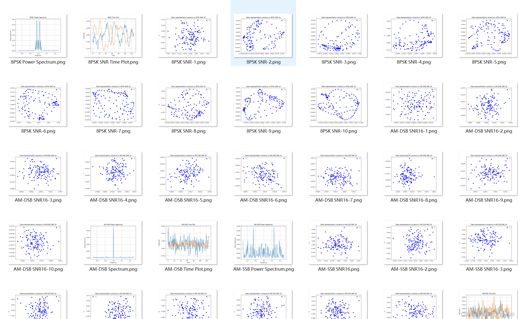
画出来的图示例:


 3681
3681

 被折叠的 条评论
为什么被折叠?
被折叠的 条评论
为什么被折叠?
 到【灌水乐园】发言


