


1、过拟台和灾拟合
过拟合是指模型能很好地拟合训练样本,但对新数据的预测准确性很差。 欠拟合是指 模型不能很好地拟合训练样本,且对新数据的预测准确性也不好。
%matplotlib inline
import matplotlib.pyplot as plt
import numpy as np

# 设置所需要的点数
n_dots = 20

# x轴的坐标
# [0, 1] 之间创建 20 个点
x = np.linspace(0, 1, n_dots)
# y轴坐标:训练样本
y = np.sqrt(x) + 0.2*np.random.rand(n_dots) - 0.1;
def plot_polynomial_fit(x, y, order):
    p = np.poly1d(np.polyfit(x, y, order))

    # 画出拟合出来的多项式所表达的曲线以及原始的点
    t = np.linspace(0, 1, 200)
    # 设置虚线和实线分别表示的模型
    plt.plot(x, y, 'ro', t, p(t), '-', t, np.sqrt(t), 'r--')
    return p
# figsize:指定figure的宽和高,单位为英寸;
plt.figure(figsize=(18, 4))
titles = ['Under Fitting', 'Fitting', 'Over Fitting']
models = [None, None, None]
for index, order in enumerate([1, 3, 10]):
    # 创建多个子图(此处为三个)
    plt.subplot(1, 3, index + 1)
    models[index] = plot_polynomial_fit(x, y, order)
    # 设置图像的标题
    plt.title(titles[index], fontsize=20)
左边是欠拟合
,也称为高偏差
,因为
我们试
图用一条直线来拟合样本数据。右边是过拟合
,也称为高方差
, 用了十阶多项式来 合数据,虽然模型对现有的数据集拟合得很好,但对新数据预测误却很大。只有中间的模型较好地拟合了数据集,可以看到虚线和实线基本
重合。
2、成本函数
成本是衡
量模型与
训练样本符合程度的指标。简单地理解,
成本
是针对
所有的训
练样
本,模型拟合出来的值与训练样本的真实值的
误差平均值
而成
本函数就是
成本与
模型参
数的函
数关系。模型
的过
程,就是找
合适
的模型
参数
,使得
成本函数的
值最小。
总结起来,针对 个数据
,我们可以选择很
个模型来拟
数据,
旦选定了某个模型,就需要从这个模型的无
穷多
个参数
找出
个最优的参数,使得成本函数的值最小。
3、模型准确性
测试数据集的成本,即J(θ) 是评估模型准确性的最直观的指标,J(θ)值越小说明模型预测出来的值与实际值差异越小,对新数据的预测准确性就越好 需要特别注意来测试模型准确性的测试数据集,必须是模型“没见过”的数据。
模型性能的不同表述方式
在scikit-learn里,不使用成本函数来表示模型的性能,而使用分数来表达,这个分数总是在[0,1]之间,数值越大说明模型的准确性越好。当模型训练完成后,调用模型的score(X_test,y_test)即可算出模型的分数值,其中X_test和y_test是测试数据集样本。模型分数与成本成反比,分数越大,准确性越高,误差越小,成本越低。
交叉验证数据集
交叉验证数据集是一个更科学的方法是把数据集分成
份,
分别是
训练数据集交叉验证数据集
测试数据集,推
荐比例是6
:
2
:2。
在模型选择
时,我们使用训
练数据集来
练算法参数
,用
交叉验证数据集来验证参数。
选择交叉验证数据集的成本 最小的多项式来作为数据拟合模型,最后再用测试数据
集来
测试选择出来的模型针对测试
数据集
的准确性。
4、学习曲线
实例
#导包
%matplotlib inline
import matplotlib.pyplot as plt
import numpy as np
n_dots = 200

X = np.linspace(0, 1, n_dots)
y = np.sqrt(X) + 0.2*np.random.rand(n_dots) - 0.1;

X = X.reshape(-1, 1)
y = y.reshape(-1, 1)

from sklearn.pipeline import Pipeline
from sklearn.preprocessing import PolynomialFeatures
from sklearn.linear_model import LinearRegression

def polynomial_model(degree=1):
    polynomial_features = PolynomialFeatures(degree=degree,
                                             include_bias=False)
    linear_regression = LinearRegression()
    pipeline = Pipeline([("polynomial_features", polynomial_features),
                         ("linear_regression", linear_regression)])
    return pipeline
from sklearn.model_selection import learning_curve
from sklearn.model_selection import ShuffleSplit

def plot_learning_curve(estimator, title, X, y, ylim=None, cv=None,
                        n_jobs=1, train_sizes=np.linspace(.1, 1.0, 5)):
     """
    Generate a simple plot of the test and training learning curve.

    Parameters
    ----------
    estimator : object type that implements the "fit" and "predict" methods
        An object of that type which is cloned for each validation.

    title : string
        Title for the chart.

    X : array-like, shape (n_samples, n_features)
        Training vector, where n_samples is the number of samples and
        n_features is the number of features.

    y : array-like, shape (n_samples) or (n_samples, n_features), optional
        Target relative to X for classification or regression;
        None for unsupervised learning.

    ylim : tuple, shape (ymin, ymax), optional
        Defines minimum and maximum yvalues plotted.

    cv : int, cross-validation generator or an iterable, optional
        Determines the cross-validation splitting strategy.
        Possible inputs for cv are:
          - None, to use the default 3-fold cross-validation,
          - integer, to specify the number of folds.
          - An object to be used as a cross-validation generator.
          - An iterable yielding train/test splits.

        For integer/None inputs, if ``y`` is binary or multiclass,
        :class:`StratifiedKFold` used. If the estimator is not a classifier
        or if ``y`` is neither binary nor multiclass, :class:`KFold` is used.

        Refer :ref:`User Guide <cross_validation>` for the various
        cross-validators that can be used here.

    n_jobs : integer, optional
        Number of jobs to run in parallel (default 1).
    """
    plt.title(title)
    if ylim is not None:
        plt.ylim(*ylim)
    plt.xlabel("Training examples")
    plt.ylabel("Score")
    train_sizes, train_scores, test_scores = learning_curve(
        estimator, X, y, cv=cv, n_jobs=n_jobs, train_sizes=train_sizes)
    train_scores_mean = np.mean(train_scores, axis=1)
    train_scores_std = np.std(train_scores, axis=1)
    test_scores_mean = np.mean(test_scores, axis=1)
    test_scores_std = np.std(test_scores, axis=1)
    plt.grid()

    plt.fill_between(train_sizes, train_scores_mean - train_scores_std,
                     train_scores_mean + train_scores_std, alpha=0.1,
                     color="r")
    plt.fill_between(train_sizes, test_scores_mean - test_scores_std,
                     test_scores_mean + test_scores_std, alpha=0.1, color="g")
    plt.plot(train_sizes, train_scores_mean, 'o--', color="r",
             label="Training score")
    plt.plot(train_sizes, test_scores_mean, 'o-', color="g",
             label="Cross-validation score")

    plt.legend(loc="best")
    return plt

# 为了让学习曲线更平滑,交叉验证数据集的得分计算 10 次,每次都重新选中 20% 的数据计算一遍
cv = ShuffleSplit(n_splits=10, test_size=0.2, random_state=0)
titles = ['Learning Curves (Under Fitting)',
          'Learning Curves',
          'Learning Curves (Over Fitting)']
degrees = [1, 3, 10]

plt.figure(figsize=(18, 4))
for i in range(len(degrees)):
    plt.subplot(1, 3, i + 1)
    plot_learning_curve(polynomial_model(degrees[i]), titles[i], X, y, ylim=(0.75, 1.01), cv=cv)

plt.show()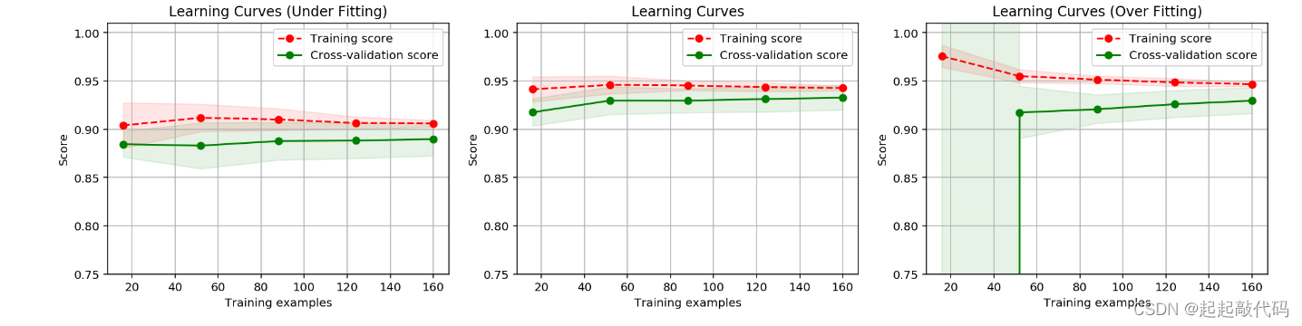
过拟合和欠拟合的特征
过拟合:模型对训练
数据集的
准确性比较
其成本
比较低
对交叉验证数
据集的准确性比较低 成本
cv
比较高
欠拟合:
模型对训练数据集的准确性
较低,其成本
较高
对交叉验证数 数据集准确性也比较 低其成本  cv
cv 比较高
比较高
5、算法模型性能优化
●获取更多的训练数据:从学习曲线的规律来看,更多的数据有助于改善过拟合问题。
减少输入的特征数量:比如,针对书写识别系统,原来使用 200 200 的图片,总
40000 个特征。优化后,我们可以把图片等比例缩小为 10 10 的图片,总共 100
个特征。这样可以大大减少模型的计算量,同时也减少模型的复杂度,改善过拟合
问题如果是欠拟合,说明模型太简单了, 需要增加模型的复杂度。
●增加有价值的特征: 重新解读并理解训练数据。比如针对 个房产价格预测的机器
学习任务,原来只根据房子面积来预测价格,结果模型出现了欠拟合。优化后,我
增加其他的特征,比如房子的朝向、户型、年代、房子旁边的学校的质量(我们
熟悉的学区房)、房子的开发商、房子周边商业街个数、房子周边公园个数等。
●增加多项式特征: 有的时候,从己知数据里挖掘出更多的特征不是件容易的事情,
这个时候,可以用纯数学的方法,增加多项式特征。


 468
468


 被折叠的 条评论
为什么被折叠?
被折叠的 条评论
为什么被折叠?
 到【灌水乐园】发言


