


《昇思25天学习打卡营第7天|CarpeDiem》
打卡
今天是昇思25天学习打卡营第7天,今天要学习的内容是 函数式自动微分
听名字就知道是用于给函数求微分的 只不过是自动的罢了
再也不用因为忘了负号寄了!!!
函数式自动微分
神经网络的训练主要使用反向传播算法,模型预测值(logits)与正确标签(label)送入损失函数(loss function)获得loss,然后进行反向传播计算,求得梯度(gradients),最终更新至模型参数(parameters)。自动微分能够计算可导函数在某点处的导数值,是反向传播算法的一般化。自动微分主要解决的问题是将一个复杂的数学运算分解为一系列简单的基本运算,该功能对用户屏蔽了大量的求导细节和过程,大大降低了框架的使用门槛。
MindSpore使用函数式自动微分的设计理念,提供更接近于数学语义的自动微分接口grad和value_and_grad。下面我们使用一个简单的单层线性变换模型进行介绍。
还是还是老样子 导入mindsproe的相关模块
import numpy as np
import mindspore
from mindspore import nn
from mindspore import ops
from mindspore import Tensor, Parameter
函数与计算图
计算图是用图论语言表示数学函数的一种方式,也是深度学习框架表达神经网络模型的统一方法。我们将根据下面的计算图构造计算函数和神经网络。
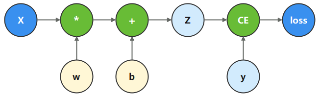
在这个模型中, x x x为输入, y y y为正确值, w w w和 b b b是我们需要优化的参数。
x = ops.ones(5, mindspore.float32)  # input tensor
y = ops.zeros(3, mindspore.float32)  # expected output
w = Parameter(Tensor(np.random.randn(5, 3), mindspore.float32), name='w') # weight
b = Parameter(Tensor(np.random.randn(3,), mindspore.float32), name='b') # bias
w w w 是一个大小为(5,3)的权重矩阵 大小即(x,y)
b b b 是一个偏置值向量 大小为(3,) 即(y,)
我们根据计算图描述的计算过程,构造计算函数。
其中,binary_cross_entropy_with_logits 是一个损失函数,计算预测值和目标值之间的二值交叉熵损失。
def function(x, y, w, b):
    z = ops.matmul(x, w) + b
    loss = ops.binary_cross_entropy_with_logits(z, y, ops.ones_like(z), ops.ones_like(z))
    return loss
binary_cross_entropy_with_logits 该函数参数:
logits (Tensor) - 输入预测值。其数据类型为float16或float32。
label (Tensor) - 输入目标值,shape与 logits 相同。数据类型为float16或float32。
weight (Tensor,可选) - 指定每个批次二值交叉熵的权重。支持广播,使其shape与 logits 的shape保持一致。数据类型必须为float16或float32。默认值:None , weight 是值为 1 的Tensor。
pos_weight (Tensor,可选) - 指定正类的权重。是一个长度等于分类数的向量。支持广播,使其shape与 logits 的shape保持一致。数据类型必须为float16或float32。默认值:None , pos_weight 是值为 1 的Tensor。
reduction (str,可选) - 指定应用于输出结果的规约计算方式,可选 ‘none’ 、 ‘mean’ 、 ‘sum’ ,默认值: ‘mean’ 。
‘none’:不应用规约方法。
‘mean’:计算输出元素的加权平均值。
‘sum’:计算输出元素的总和。
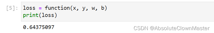
执行计算函数,可以获得计算的loss值。
loss = function(x, y, w, b)
print(loss)
微分函数与梯度计算
为了优化模型参数,需要求参数对loss的导数:
∂
loss
∂
w
\frac{\partial \operatorname{loss}}{\partial w}
∂w∂loss和
∂
loss
∂
b
\frac{\partial \operatorname{loss}}{\partial b}
∂b∂loss,此时我们调用mindspore.grad函数,来获得function的微分函数。
这里使用了grad函数的两个入参,分别为:
fn:待求导的函数。grad_position:指定求导输入位置的索引。
由于我们对
w
w
w和
b
b
b求导,因此配置其在function入参对应的位置(2, 3)。
使用
grad获得微分函数是一种函数变换,即输入为函数,输出也为函数。
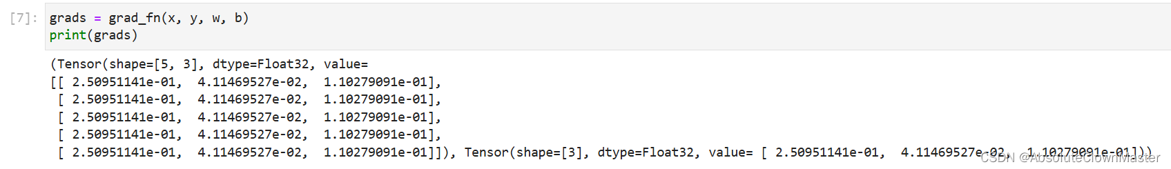
grad_fn = mindspore.grad(function, (2, 3))
执行微分函数,即可获得 w w w、 b b b对应的梯度。
grads = grad_fn(x, y, w, b)
print(grads)
Stop Gradient
通常情况下,求导时会求loss对参数的导数,因此函数的输出只有loss一项。当我们希望函数输出多项时,微分函数会求所有输出项对参数的导数。此时如果想实现对某个输出项的梯度截断,或消除某个Tensor对梯度的影响,需要用到Stop Gradient操作。
这里我们将function改为同时输出loss和z的function_with_logits,获得微分函数并执行。
def function_with_logits(x, y, w, b):
    z = ops.matmul(x, w) + b
    loss = ops.binary_cross_entropy_with_logits(z, y, ops.ones_like(z), ops.ones_like(z))
    return loss, z
grad_fn = mindspore.grad(function_with_logits, (2, 3))
grads = grad_fn(x, y, w, b)
print(grads)
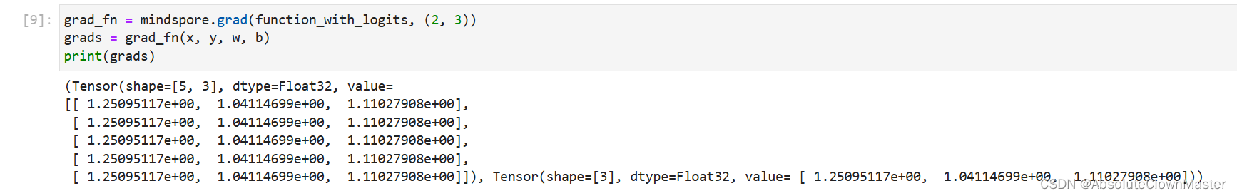
可以看到求得
w
w
w、
b
b
b对应的梯度值发生了变化。此时如果想要屏蔽掉z对梯度的影响,即仍只求参数对loss的导数,可以使用ops.stop_gradient接口,将梯度在此处截断。我们将function实现加入stop_gradient,并执行。
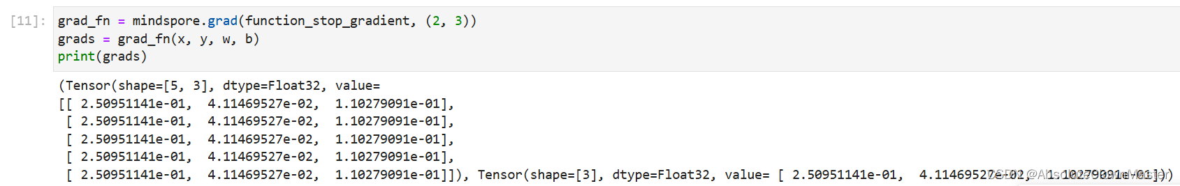
def function_stop_gradient(x, y, w, b):
    z = ops.matmul(x, w) + b
    loss = ops.binary_cross_entropy_with_logits(z, y, ops.ones_like(z), ops.ones_like(z))
    return loss, ops.stop_gradient(z)
grad_fn = mindspore.grad(function_stop_gradient, (2, 3))
grads = grad_fn(x, y, w, b)
print(grads)
matmul 执行矩阵乘法 矩阵形状为 (n,m) (m,p) 最后相乘得到的矩阵形状为 (n,p)
可以看到,求得
w
w
w、
b
b
b对应的梯度值与初始function求得的梯度值一致。
Auxiliary data
Auxiliary data意为辅助数据,是函数除第一个输出项外的其他输出。通常我们会将函数的loss设置为函数的第一个输出,其他的输出即为辅助数据。
grad和value_and_grad提供has_aux参数,当其设置为True时,可以自动实现前文手动添加stop_gradient的功能,满足返回辅助数据的同时不影响梯度计算的效果。
下面仍使用function_with_logits,配置has_aux=True,并执行。
grad_fn = mindspore.grad(function_with_logits, (2, 3), has_aux=True)
grads, (z,) = grad_fn(x, y, w, b)
print(grads, z)
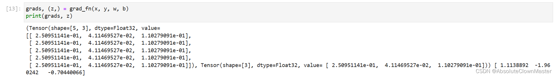
可以看到,求得
w
w
w、
b
b
b对应的梯度值与初始function求得的梯度值一致,同时z能够作为微分函数的输出返回。
神经网络梯度计算
前述章节主要根据计算图对应的函数介绍了MindSpore的函数式自动微分,但我们的神经网络构造是继承自面向对象编程范式的nn.Cell。接下来我们通过Cell构造同样的神经网络,利用函数式自动微分来实现反向传播。
首先我们继承nn.Cell构造单层线性变换神经网络。这里我们直接使用前文的
w
w
w、
b
b
b作为模型参数,使用mindspore.Parameter进行包装后,作为内部属性,并在construct内实现相同的Tensor操作。
# Define model
class Network(nn.Cell):
    def __init__(self):
        super().__init__()
        self.w = w
        self.b = b

    def construct(self, x):
        z = ops.matmul(x, self.w) + self.b
        return z
接下来我们实例化模型(model)和损失函数(loss_fn)。
# Instantiate model
model = Network()
# Instantiate loss function
loss_fn = nn.BCEWithLogitsLoss()
nn.BCEWithLogitsLoss() 这个函数是用于二分类问题的损失函数 结合了 Sigmoid 激活函数和二进制交叉熵(BCE)损失
完成后,由于需要使用函数式自动微分,需要将神经网络和损失函数的调用封装为一个前向计算函数。
# Define forward function
def forward_fn(x, y):
    z = model(x)
    loss = loss_fn(z, y)
    return loss
完成后,我们使用value_and_grad接口获得微分函数,用于计算梯度。
由于使用Cell封装神经网络模型,模型参数为Cell的内部属性,此时我们不需要使用grad_position指定对函数输入求导,因此将其配置为None。对模型参数求导时,我们使用weights参数,使用model.trainable_params()方法从Cell中取出可以求导的参数。
grad_fn = mindspore.value_and_grad(forward_fn, None, weights=model.trainable_params())
以下是 mindspore.value_and_grad() 函数的解释
Signature: mindspore.value_and_grad(fn, grad_position=0, weights=None, has_aux=False)Docstring:
A wrapper function to generate the function to calculate forward output and gradient for the input function.
As for gradient, three typical cases are included:
gradient with respect to inputs. In this case,
grad_positionis not None whileweightsis None.gradient with respect to weights. In this case,
grad_positionis None whileweightsis not None.gradient with respect to inputs and weights. In this case,
grad_positionandweightsare not None.Args:
fn (Union[Cell, Function]): Function to do GradOperation.
grad_position (Union[NoneType, int, tuple[int]]): Index to specify which inputs to be differentiated.
If int, get the gradient with respect to single input.
If tuple, get the gradients with respect to selected inputs.grad_positionbegins with 0.
If None, none derivative of any input will be solved, and in this case,weightsis required.
Default:0.weights (Union[ParameterTuple, Parameter, list[Parameter]]): The parameters of the training network that need to
calculate the gradient.weightscan be got throughweights = net.trainable_params().
Default:None.has_aux (bool): If
True, only the first output offncontributes the gradient offn, while the other
outputs will be returned straightly. It means thefnmust return more than one outputs in this case.
Default:False.Returns:
Function, returns the gradient function to calculate forward output and gradient for the input function or cell.
For example, as forout1, out2 = fn(*args), gradient function will return outputs like
((out1, out2), gradient). Whenhas_auxis set True, onlyout1contributes to the differentiation.
loss, grads = grad_fn(x, y)
print(grads)
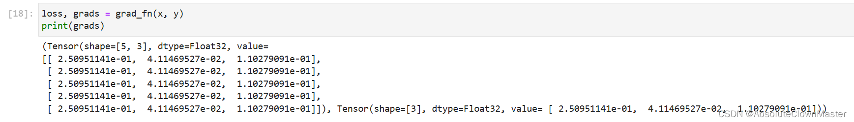
执行微分函数,可以看到梯度值和前文function求得的梯度值一致。
今天学习的函数式自动微分,可以帮助我们节省到很多求导方面的工作,只需要一个grad的函数变化就可以帮助我们实现求函数导数的功能,相交自己手动用代码实现一个求导的功能可谓是方便了不少


 1125
1125

 被折叠的 条评论
为什么被折叠?
被折叠的 条评论
为什么被折叠?
 到【灌水乐园】发言


