PyTorch学习笔记-3.PyTorch模型搭建

3.PyTorch模型搭建

3.1.卷积层

3.1.1.卷积-1d/2d/3d

卷积运算：卷积核在输入信号（图像）上滑动，相应位置上进行乘加
卷积核：又称为滤波器，过滤器，可认为是某种模式，某种特征。

卷积过程类似于用一个模版去图像上寻找与它相似的区域，与卷积核模式越相似，激活值越高，从而实现特征提取

例如：

AlexNet卷积核可视化，发现卷积核学习到的是边缘，条纹，色彩这一些细节模式

卷积维度： 一般情况下，卷积核在几个维度上滑动，就是几维卷积

下面分别为一维、二维、三维卷积示意图

 

通常，我们常用的为二维卷积，如何生成二维卷积？

nn.Conv2d

功能：对多个二维信号进行二维卷积
• in_channels：输入通道数
• out_channels：输出通道数，等价于卷积核个数
• kernel_size：卷积核尺寸
• stride：步长
• padding ：填充个数

• dilation：空洞卷积大小
• groups：分组卷积设置
• bias：偏置

nn.Conv2d(in_channels,
out_channels,
kernel_size,
stride=1,
padding=0,
dilation=1,
groups=1,
bias=True,
padding_mode='zeros') 

padding：

 

空洞卷积大小：

分组卷积：例如AlexNet，分为两组

卷积后的尺寸计算：

代码实现：

利用二维卷积提取图片特征

# -*- coding: utf-8 -*-
import os
import torch
import random
import numpy as np
import torch.nn as nn
from PIL import Image
from torchvision import transforms
from matplotlib import pyplot as plt

def transform_invert(img_, transform_train):
    """
    将data 进行反transfrom操作
    :param img_: tensor
    :param transform_train: torchvision.transforms
    :return: PIL image
    """
    if 'Normalize' in str(transform_train):
        norm_transform = list(filter(lambda x: isinstance(x, transforms.Normalize), transform_train.transforms))
        mean = torch.tensor(norm_transform[0].mean, dtype=img_.dtype, device=img_.device)
        std = torch.tensor(norm_transform[0].std, dtype=img_.dtype, device=img_.device)
        img_.mul_(std[:, None, None]).add_(mean[:, None, None])

    img_ = img_.transpose(0, 2).transpose(0, 1)  # C*H*W --> H*W*C
    if 'ToTensor' in str(transform_train):
        img_ = img_.detach().numpy() * 255

    if img_.shape[2] == 3:
        img_ = Image.fromarray(img_.astype('uint8')).convert('RGB')
    elif img_.shape[2] == 1:
        img_ = Image.fromarray(img_.astype('uint8').squeeze())
    else:
        raise Exception("Invalid img shape, expected 1 or 3 in axis 2, but got {}!".format(img_.shape[2]) )

    return img_

def set_seed(seed=1):
    random.seed(seed)
    np.random.seed(seed)
    torch.manual_seed(seed)
    torch.cuda.manual_seed(seed)

set_seed(1)  # 设置随机种子

# 数据加载
# os.path.dirname(__file__)返回的是.py文件的目录
path_img = os.path.join(os.path.dirname(__file__), "lena.png")
img = Image.open(path_img).convert('RGB')  # 0~255

# convert to tensor
img_transform = transforms.Compose([transforms.ToTensor()])
img_tensor = img_transform(img)
img_tensor.unsqueeze_(dim=0)    # C*H*W to B*C*H*W

# 创建卷积层Conv2d
# 设置卷积层输入channel为3，卷积核数量为1，卷积核大小为3
conv_layer = nn.Conv2d(3, 1, 3)
# 初始化权重，即卷积核，conv_layer.weight.data返回权重（卷积核）的shape，(卷积核数量, 深度，高, 宽)
# nn.init.xavier_normal_为Xavier正态分布初始化，参数由0均值，标准差为sqrt(2 / (fan_in + fan_out))的正态分布产生
# 其中fan_in和fan_out是分别权值张量的输入和输出元素数目. 这种初始化同样是为了保证输入输出的方差不变
# 在tanh激活函数上有很好的效果，但不适用于ReLU激活函数
nn.init.xavier_normal_(conv_layer.weight.data)

# calculation
img_conv = conv_layer(img_tensor)

# 可视化
print("卷积前尺寸:{}\n卷积后尺寸:{}".format(img_tensor.shape, img_conv.shape))
# 对卷积后的图像进行逆变换，卷积后只有一个通道
img_conv = transform_invert(img_conv[0, 0:1, ...], img_transform)
img_raw = transform_invert(img_tensor.squeeze(), img_transform)
plt.subplot(121).imshow(img_raw)
plt.subplot(122).imshow(img_conv, cmap='gray')
plt.show()

卷积前尺寸:torch.Size([1, 3, 512, 512]) 卷积后尺寸:torch.Size([1, 1, 510, 510])

上例中，卷积核的shape为(1,3,3,3)，表示一个卷积核，3个通道，高、宽都是3

卷积维度： 一般情况下，卷积核在几个维度上滑动，就是几维卷积

如图：卷积核是在一个二维数据上滑动，就是二维卷积

其中红色卷积核只在第一个通道上滑动

最后得到的结果是由三个卷积核与对应位置的乘加后的结果再次相加而得

3.1.2.转置卷积

转置卷积 用于对图像进行上采样(UpSample)

正常卷积：
假设图像尺寸为4*4，卷积核为3*3， padding=0， stride=1

转置卷积：
假设图像尺寸为2*2，卷积核为3*3， padding=0， stride=1

下图分别为正常卷积和转置卷积示意图：

 

转置卷积核卷积的方法参数类似：

nn.ConvTranspose2d
功能：转置卷积实现上采样
• in_channels：输入通道数
• out_channels：输出通道数
• kernel_size：卷积核尺寸
• stride：步长
• padding ：填充个数

• dilation：空洞卷积大小
• groups：分组卷积设置
• bias：偏置

nn.ConvTranspose2d(in_channels,
out_channels,
kernel_size,
stride=1,
padding=0,
output_padding=0,
groups=1,
bias=True,
dilation=1,
padding_mode='zeros') 

尺寸计算：

代码实现：

# 创建转置卷积层ConvTranspose2d

conv_layer = nn.ConvTranspose2d(3, 1, 3, stride=2)   # input:(i, o, size)
nn.init.xavier_normal_(conv_layer.weight.data)

# calculation
img_conv = conv_layer(img_tensor)

卷积前尺寸:torch.Size([1, 3, 512, 512]) 卷积后尺寸:torch.Size([1, 1, 1025, 1025])

3.2.池化层

池化运算：对信号进行 “收集”并 “总结”，类似水池收集水资源，因而得名池化层

“收集”：多变少 “总结”：最大值/平均值

 

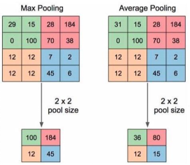
池化方法：

nn.MaxPool2d

功能：对二维信号（图像）进行最大值池化
• kernel_size：池化核尺寸
• stride：步长
• padding ：填充个数
• dilation：池化核间隔大小
• ceil_mode：尺寸向上取整
• return_indices：记录池化像素索引

nn.MaxPool2d(kernel_size,

stride=None,
padding=0,

dilation=1,
ceil_mode=False,

return_indices=False) 

代码实现：

将卷积层的创建代码改为池化层即可（注意变量的命名，最后可视化的时候需要一致）

# 创建池化层MaxPool2d

# 最大值池化，stride=(2, 2)表示向右和向下步长都是2
maxpool_layer = nn.MaxPool2d((2, 2), stride=(2, 2))
img_pool = maxpool_layer(img_tensor)

池化前尺寸:torch.Size([1, 3, 512, 512]) 池化后尺寸:torch.Size([1, 3, 256, 256])

nn.AvgPool2d

功能：对二维信号（图像）进行平均值池化
• kernel_size：池化核尺寸
• stride：步长
• padding ：填充个数
• ceil_mode：尺寸向上取整
• count_include_pad：填充值用于计算
• divisor_override ：除法因子，正常是除以池化尺寸像素的数量，这里可以自定义

nn.AvgPool2d(kernel_size,
stride=None,
padding=0,
ceil_mode=False,
count_include_pad=True,
divisor_override=None) 

代码实现：

# 创建池化层AvgPool2d

avgpoollayer = nn.AvgPool2d((2, 2), stride=(2, 2))
img_pool = avgpoollayer(img_tensor)

池化前尺寸:torch.Size([1, 3, 512, 512]) 池化后尺寸:torch.Size([1, 3, 256, 256])

# 创建池化层AvgPool2d ，设置除法因子divisor_override

img_tensor = torch.ones((1, 1, 4, 4))
avgpool_layer = nn.AvgPool2d((2, 2), stride=(2, 2), divisor_override=3)
img_pool = avgpool_layer(img_tensor)

print("raw_img:\n{}\npooling_img:\n{}".format(img_tensor, img_pool))

raw_img: tensor([[[[1., 1., 1., 1.],           [1., 1., 1., 1.],           [1., 1., 1., 1.],           [1., 1., 1., 1.]]]]) pooling_img: tensor([[[[1.3333, 1.3333],           [1.3333, 1.3333]]]])

 

反池化方法：

nn.MaxUnpool2d

功能：对二维信号（图像）进行最大值池化上采样

• kernel_size：池化核尺寸
• stride：步长
• padding ：填充个数

nn.MaxUnpool2d(kernel_size,
stride=None,
padding=0) 

代码实现：

# 创建池化层，然后进行反池化

img_tensor = torch.randint(high=5, size=(1, 1, 4, 4), dtype=torch.float)
maxpool_layer = nn.MaxPool2d((2, 2), stride=(2, 2), return_indices=True)
img_pool, indices = maxpool_layer(img_tensor)

# unpooling
maxunpool_layer = nn.MaxUnpool2d((2, 2), stride=(2, 2))
img_unpool = maxunpool_layer(img_pool, indices)

print("raw_img:\n{}\nimg_pool:\n{}".format(img_tensor, img_pool))
print("img_unpool:\n{}".format(img_unpool))

3.3线性层

线性层又称全连接层，其每个神经元与上一层所有神经元相连实现对前一层的线性组合， 线性变换

例如：

Input=[1, 2, 3] shape=(1, 3)

 shape=(3,4)

Hidden = Input×W_0=[6, 12, 18, 24] shape=(1,4)

构建线性层：

nn.Linear

功能：对一维信号（向量）进行线性组合
• in_features：输入结点数
• out_features：输出结点数
• bias ：是否需要偏置
计算公式：

nn.Linear(in_features, out_features, bias=True) 

代码实现：

# 创建线性层

inputs = torch.tensor([[1., 2, 3]])
# 线性层，输入大小为3，输出大小为4
linear_layer = nn.Linear(3, 4)
linear_layer.weight.data = torch.tensor([[1., 1., 1.],
                                 [2., 2., 2.],
                                 [3., 3., 3.],
                                 [4., 4., 4.]])
# 设置bias
linear_layer.bias.data.fill_(0.5)
output = linear_layer(inputs)
print(inputs, inputs.shape)
print(linear_layer.weight.data, linear_layer.weight.data.shape)
print(output, output.shape)

tensor([[1., 2., 3.]]) torch.Size([1, 3]) tensor([[1., 1., 1.],         [2., 2., 2.],         [3., 3., 3.],         [4., 4., 4.]]) torch.Size([4, 3]) tensor([[ 6.5000, 12.5000, 18.5000, 24.5000]], grad_fn=<AddmmBackward>) torch.Size([1, 4])

3.4.激活函数层

激活函数对特征进行非线性变换，赋予多层神经网络具有深度的意义

如果没有激活函数，多个线性变换等价于一个线性变换

例如：

 

常用的激活函数：

nn.Sigmoid

计算公式：

梯度公式：

特性：
• 输出值在(0,1)，符合概率
• 导数范围是[0, 0.25],易导致梯度消失
• 输出为非0均值，破坏数据分布

nn.tanh

计算公式：

梯度公式：

特性：
• 输出值在(-1,1)，数据符合0均值
• 导数范围是(0, 1),易导致梯度消失

nn.ReLU

计算公式：

梯度公式：

特性：

• 解决了梯度消失、爆炸的问题

• 计算方便，计算速度快

• 加速了网络的训练

• 输出值均为正数，负半轴导致死神经元

• 输出不是以0为均值 

针对ReLU的改进：

nn.LeakyReLU

• negative_slope: 负半轴斜率  

nn.PReLU

• init: 可学习斜率

nn.RReLU

• lower: 均匀分布下限
• upper:均匀分布上限

3.5.模型构建

3.5.1.自定义模型

pytorch中模型的构建是通过类来构建的

模型搭建三要素：

1.必须要继承nn.Module这个类，要让PyTorch知道这个类是一个Module

2.在__init__(self)中设置好需要的组件，比如conv，pooling，Linear等等

3.最后在forward(self,x)中用定义好的组件进行组装，就像搭积木，把网络结构搭建出来，这样一个模型就定义好了

 

以LeNet为例构建模型

LeNet：Conv1->pool1->Conv2->pool2->fc1->fc2->fc3

LeNet执行过程：

 

代码实现：

# -*- coding: utf-8 -*-
import torch
import torch.nn as nn
from collections import OrderedDict
import torch.nn.functional as F

class LeNet(nn.Module):
    def __init__(self, classes):
        super(LeNet, self).__init__()
        self.conv1 = nn.Conv2d(3, 6, 5)
        self.conv2 = nn.Conv2d(6, 16, 5)
        self.fc1 = nn.Linear(16*5*5, 120)
        self.fc2 = nn.Linear(120, 84)
        self.fc3 = nn.Linear(84, classes)

    def forward(self, x):
        # F为具体实现的函数，上面的直接调用nn.ReLU() 为类，而F.relu()为函数
        out = F.relu(self.conv1(x))
        out = F.max_pool2d(out, 2)
        out = F.relu(self.conv2(out))
        out = F.max_pool2d(out, 2)
        # 将上面的结果拉伸为一行，其中第一个out.size(0)表示批大小，后面-1表示将多个维度的数据拉伸为一个维度，大小自适应

# view()函数返回和原tensor数据个数相同，但size不同的tensor
        # 例如：输入为16*32*7*7，输出即16*1568
        out = out.view(out.size(0), -1)
        out = F.relu(self.fc1(out))
        out = F.relu(self.fc2(out))
        out = self.fc3(out)
        return out

# 创建模型，设置最终输出为2分类
net = LeNet(classes=2)

#随机生成图像数据
fake_img = torch.randn((4, 3, 32, 32), dtype=torch.float32)
output = net(fake_img)

print(net)
print(output.shape)
print(output)

LeNet(   (conv1): Conv2d(3, 6, kernel_size=(5, 5), stride=(1, 1))   (conv2): Conv2d(6, 16, kernel_size=(5, 5), stride=(1, 1))   (fc1): Linear(in_features=400, out_features=120, bias=True)   (fc2): Linear(in_features=120, out_features=84, bias=True)   (fc3): Linear(in_features=84, out_features=2, bias=True) ) torch.Size([4, 2]) tensor([[0.0571, 0.0786],         [0.0567, 0.0706],         [0.0481, 0.0788],         [0.0320, 0.0534]], grad_fn=<AddmmBackward>)

 

3.5.2.通过容器构建模型

nn.Sequential 是 nn.module的容器，用于按顺序包装一组网络层
例如：

可以将LeNet结构的卷积和池化放在一个容器中，作为提取特征的容器

将全连接层放入另一个容器中，作为分类层

 

代码实现：

# -*- coding: utf-8 -*-
import torch
import torch.nn as nn
from collections import OrderedDict
import torch.nn.functional as F

# 通过Sequential构建模型
class LeNetSequential(nn.Module):
    def __init__(self, classes):
        super(LeNetSequential, self).__init__()
        self.features = nn.Sequential(
            nn.Conv2d(3, 6, 5),
            nn.ReLU(),
            nn.MaxPool2d(kernel_size=2, stride=2),
            nn.Conv2d(6, 16, 5),
            nn.ReLU(),
            nn.MaxPool2d(kernel_size=2, stride=2),)

        self.classifier = nn.Sequential(
            nn.Linear(16*5*5, 120),
            nn.ReLU(),
            nn.Linear(120, 84),
            nn.ReLU(),
            nn.Linear(84, classes),)

    def forward(self, x):
        x = self.features(x)
        x = x.view(x.size()[0], -1)
        x = self.classifier(x)
        return x

# 创建模型，设置最终输出为2分类
net = LeNetSequential(classes=2)

#随机生成图像数据
fake_img = torch.randn((4, 3, 32, 32), dtype=torch.float32)
output = net(fake_img)

print(net)
print(output.shape)
print(output)

LeNetSequential(   (features): Sequential(     (0): Conv2d(3, 6, kernel_size=(5, 5), stride=(1, 1))     (1): ReLU()     (2): MaxPool2d(kernel_size=2, stride=2, padding=0, dilation=1, ceil_mode=False)     (3): Conv2d(6, 16, kernel_size=(5, 5), stride=(1, 1))     (4): ReLU()     (5): MaxPool2d(kernel_size=2, stride=2, padding=0, dilation=1, ceil_mode=False)   )   (classifier): Sequential(     (0): Linear(in_features=400, out_features=120, bias=True)     (1): ReLU()     (2): Linear(in_features=120, out_features=84, bias=True)     (3): ReLU()     (4): Linear(in_features=84, out_features=2, bias=True)   ) ) torch.Size([4, 2]) tensor([[ 7.1048e-03, -1.2472e-01],         [-7.2047e-06, -1.2855e-01],         [-1.3151e-02, -1.5279e-01],         [-6.2594e-04, -1.4584e-01]], grad_fn=<AddmmBackward>)

 

直接使用Sequential构建模型时，每层的index为序号，可以使用字典为每层定义名称

实现代码：

# -*- coding: utf-8 -*-
import torch
import torch.nn as nn
from collections import OrderedDict
import torch.nn.functional as F

class LeNetSequentialOrderDict(nn.Module):
    def __init__(self, classes):
        super(LeNetSequentialOrderDict, self).__init__()

        self.features = nn.Sequential(OrderedDict({
            'conv1': nn.Conv2d(3, 6, 5),
            'relu1': nn.ReLU(inplace=True),
            'pool1': nn.MaxPool2d(kernel_size=2, stride=2),

            'conv2': nn.Conv2d(6, 16, 5),
            'relu2': nn.ReLU(inplace=True),
            'pool2': nn.MaxPool2d(kernel_size=2, stride=2),
        }))

        self.classifier = nn.Sequential(OrderedDict({
            'fc1': nn.Linear(16*5*5, 120),
            'relu3': nn.ReLU(),

            'fc2': nn.Linear(120, 84),
            'relu4': nn.ReLU(inplace=True),

            'fc3': nn.Linear(84, classes),
        }))

    def forward(self, x):
        x = self.features(x)
        x = x.view(x.size()[0], -1)
        x = self.classifier(x)
        return x

# 创建模型，设置最终输出为2分类
net = LeNetSequentialOrderDict(classes=2)

#随机生成图像数据
fake_img = torch.randn((4, 3, 32, 32), dtype=torch.float32)
output = net(fake_img)

print(net)
print(output.shape)
print(output)

LeNetSequentialOrderDict(   (features): Sequential(     (conv1): Conv2d(3, 6, kernel_size=(5, 5), stride=(1, 1))     (relu1): ReLU(inplace=True)     (pool1): MaxPool2d(kernel_size=2, stride=2, padding=0, dilation=1, ceil_mode=False)     (conv2): Conv2d(6, 16, kernel_size=(5, 5), stride=(1, 1))     (relu2): ReLU(inplace=True)     (pool2): MaxPool2d(kernel_size=2, stride=2, padding=0, dilation=1, ceil_mode=False)   )   (classifier): Sequential(     (fc1): Linear(in_features=400, out_features=120, bias=True)     (relu3): ReLU()     (fc2): Linear(in_features=120, out_features=84, bias=True)     (relu4): ReLU(inplace=True)     (fc3): Linear(in_features=84, out_features=2, bias=True)   ) ) torch.Size([4, 2]) tensor([[-0.1009, -0.1435],         [-0.0963, -0.1385],         [-0.0813, -0.1394],         [-0.1012, -0.1286]], grad_fn=<AddmmBackward>)

 

nn.ModuleList是 nn.module的容器，用于包装一组网络层，以迭代方式调用网络层

主要方法：
• append()： 在ModuleList后面添加网络层
• extend()：拼接两个ModuleList
• insert()： 指定在ModuleList中位置插入网络层

代码实现：

class ModuleList(nn.Module):
    def __init__(self):
        super(ModuleList, self).__init__()
        # 创建20层的线性层
        self.linears = nn.ModuleList([nn.Linear(10, 10) for i in range(20)])

    def forward(self, x):
        for i, linear in enumerate(self.linears):
            x = linear(x)
        return x

net = ModuleList()
print(net)

fake_data = torch.ones((10, 10))
output = net(fake_data)

print(output)

ModuleList(   (linears): ModuleList(     (0): Linear(in_features=10, out_features=10, bias=True)     (1): Linear(in_features=10, out_features=10, bias=True)              ...     (19): Linear(in_features=10, out_features=10, bias=True)   ) ) tensor([[-0.4264,  0.2802, -0.0323,  0.0848,  0.1402, -0.1814, -0.1415,  0.3992,           0.1497,  0.0838],         [-0.4264,  0.2802, -0.0323,  0.0848,  0.1402, -0.1814, -0.1415,  0.3992,           0.1497,  0.0838],                     ...         [-0.4264,  0.2802, -0.0323,  0.0848,  0.1402, -0.1814, -0.1415,  0.3992,           0.1497,  0.0838]], grad_fn=<AddmmBackward>)

 

最后，可以通过所学知识，查看AlexNet模型

AlexNet模型介绍：

AlexNet： 2012年以高出第二名10多个百分点的准确率获得ImageNet分类任务冠军，开创了卷积神经网络的新时代，架构图如下：

可以通过点击AlexNet查看源代码

import torchvision

alexnet = torchvision.models.AlexNet()

 

AlexNet创建的源代码：

import torch
import torch.nn as nn

class AlexNet(nn.Module):

    def __init__(self, num_classes=1000):
        super(AlexNet, self).__init__()
        self.features = nn.Sequential(
            nn.Conv2d(3, 64, kernel_size=11, stride=4, padding=2),
            nn.ReLU(inplace=True),
            nn.MaxPool2d(kernel_size=3, stride=2),
            nn.Conv2d(64, 192, kernel_size=5, padding=2),
            nn.ReLU(inplace=True),
            nn.MaxPool2d(kernel_size=3, stride=2),
            nn.Conv2d(192, 384, kernel_size=3, padding=1),
            nn.ReLU(inplace=True),
            nn.Conv2d(384, 256, kernel_size=3, padding=1),
            nn.ReLU(inplace=True),
            nn.Conv2d(256, 256, kernel_size=3, padding=1),
            nn.ReLU(inplace=True),
            nn.MaxPool2d(kernel_size=3, stride=2),
        )
        self.avgpool = nn.AdaptiveAvgPool2d((6, 6))
        self.classifier = nn.Sequential(
            nn.Dropout(),
            nn.Linear(256 * 6 * 6, 4096),
            nn.ReLU(inplace=True),
            nn.Dropout(),
            nn.Linear(4096, 4096),
            nn.ReLU(inplace=True),
            nn.Linear(4096, num_classes),
        )

    def forward(self, x):
        x = self.features(x)
        x = self.avgpool(x)
        x = torch.flatten(x, 1)
        x = self.classifier(x)
        return x