Frobenius product

Hadamard product
Main article: Hadamard product (matrices)
For two matrices of the same dimensions, there is the Hadamard product, also known as the element-wise product, pointwise product, entrywise product and the Schur product.[24] For two matrices A and B of the same dimensions, the Hadamard product A ○ B is a matrix of the same dimensions, the i, j element of A is multiplied with the i, j element of B, that is:

$$\left(\mathbf{A} \circ \mathbf{B}\right)_{ij} = A_{ij}B_{ij}$$
displayed fully:

$$\mathbf{A} \circ \mathbf{B} = \begin{pmatrix} A_{11} & A_{12} & \cdots & A_{1m} \\ A_{21} & A_{22} & \cdots & A_{2m} \\ \vdots & \vdots & \ddots & \vdots \\ A_{n1} & A_{n2} & \cdots & A_{nm} \\ \end{pmatrix}\circ\begin{pmatrix} B_{11} & B_{12} & \cdots & B_{1m} \\ B_{21} & B_{22} & \cdots & B_{2m} \\ \vdots & \vdots & \ddots & \vdots \\ B_{n1} & B_{n2} & \cdots & B_{nm} \\ \end{pmatrix} =\begin{pmatrix} A_{11}B_{11} & A_{12}B_{12} & \cdots & A_{1m}B_{1m} \\ A_{21}B_{21} & A_{22}B_{22} & \cdots & A_{2m}B_{2m} \\ \vdots & \vdots & \ddots & \vdots \\ A_{n1}B_{n1} & A_{n2}B_{n2} & \cdots & A_{nm}B_{nm} \\ \end{pmatrix}$$
This operation is identical to multiplying many ordinary numbers (mn of them) all at once; thus the Hadamard product is commutative, associative and distributive over entrywise addition. It is also a principal submatrix of the Kronecker product. It appears in lossy compression algorithms such as JPEG.

Frobenius product
The Frobenius inner product, sometimes denoted A : B, is the component-wise inner product of two matrices as though they are vectors. It is also the sum of the entries of the Hadamard product. Explicitly,

$$\mathbf{A}:\mathbf{B}=\sum_{i,j} A_{ij} B_{ij} = \mathrm{vec}(\mathbf{A})^\mathsf{T} \mathrm{vec}(\mathbf{B}) = \mathrm{tr}(\mathbf{A}^\mathsf{T} \mathbf{B}) = \mathrm{tr}(\mathbf{A} \mathbf{B}^\mathsf{T}),$$
where “tr” denotes the trace of a matrix and vec denotes vectorization. This inner product induces the Frobenius norm.

$\mathbf{A}:\mathbf{B}=\mathbf{B}:\mathbf{A}$

$\mathbf{A}:\mathbf{B}=\mathbf{A^T}:\mathbf{B^T}=\mathbf{B^T}:\mathbf{A^T}$

$\mathbf{A}:\mathbf{BC}=\mathbf{B^TA}:\mathbf{C}$

$\mathbf{A}:\mathbf{BC}=\mathbf{AC^T}:\mathbf{B}$

$\mathbf{A}:\mathbf{(B+C)}=\mathbf{A:B}+\mathbf{A:C}$

$\nabla(\mathbf{A}:\mathbf{B})=\nabla\mathbf{A}:\mathbf{B}+\mathbf{A}:\nabla\mathbf{B}$
(证明如下:

$$\begin{align} \nabla(\mathbf{A}:\mathbf{B}) &=\nabla(\sum_{i,j} A_{ij} B_{ij}) \hspace{800px} \\ & = \sum_{i,j}(\nabla (A_{ij} B_{ij}))\\ & = \sum_{i,j}(\nabla A_{ij} B_{ij} + A_{ij} \nabla B_{ij}) \\ & = \sum_{i,j}(\nabla A_{ij}B_{ij})+\sum_{i,j}( A_{ij}\nabla B_{ij})\\ & =\nabla\mathbf{A}:\mathbf{B}+\mathbf{A}:\nabla\mathbf{B} \end{align}$$
)

另外,关于导数

$$\frac{d(\mathbf{A}:\mathbf{X})}{d\mathbf{X}} = \frac{d(\mathbf{X}:\mathbf{A})}{d\mathbf{X}} = \mathbf{1} \circ \mathbf{A}=\mathbf{A}$$

证明一下

$$\begin{align*} &\frac{d(\mathbf{A}:\mathbf{X})}{d\mathbf{X}} = \frac{d(\mathbf{X}:\mathbf{A})}{d\mathbf{X}} = \frac{d(\sum_{i,j}\mathbf A_{i,j}\mathbf X_{i,j})}{\mathbf X}&\\ &\frac{d(\mathbf{A}:\mathbf{X})}{d\mathbf{X}_{i,j}} = \frac{d(\mathbf{X}:\mathbf{A})}{d\mathbf{X}_{i,j}} = \frac{d(\sum_{i,j}\mathbf A_{i,j}\mathbf X_{i,j})}{d\mathbf X_{i,j}}=A_{i,j} * 1& \end{align*}$$

同理

$$\begin{align*} &\frac{d(\mathbf{A}:\mathbf{F(X)})}{d\mathbf{X}} = \frac{d(\sum_{i,j}\mathbf A_{i,j}\mathbf F_{i,j})}{\mathbf X}&\\ &\frac{d(\mathbf{A}:\mathbf{F})}{d\mathbf{X}_{i,j}} = \frac{d(\sum_{i,j}\mathbf A_{i,j}\mathbf F_{i,j})}{d\mathbf X_{i,j}}=A_{i,j} * \frac{d\mathbf F_{i,j}}{d\mathbf X_{i,j}}&\\ &所以&\\ &\frac{d(\mathbf{A}:\mathbf{F})}{d\mathbf{X}} = \mathbf A \circ \frac{d\mathbf F}{d\mathbf X} \end{align*}$$
其中 求导和最后的合并都是elementwise的

对于二阶导数的求法, 这里只推导matrix cookbook上的一个公式(110), 其他的类似

$$\frac{\partial}{\partial X}\mathrm{tr}(\mathbf{X}\mathbf{X^T}\mathbf{B}) = \mathbf{B}\mathbf{X}+\mathbf{B^T}\mathbf{X}$$

求导的方法,相办法把每个$\mathbf{X}$单独写在$:$的一边, 为了区别两个$\mathbf{X}$, 我把它们分别表示为$\mathbf{X_1}$,$\mathbf{X_2}$

$$\begin{align} &\nabla\mathrm{tr}(\mathbf{X_1}\mathbf{X_2^T}\mathbf{B}) = \nabla(\mathbf{X_1}:\mathbf{B^TX_2})=\nabla\mathbf{X_1}:\mathbf{B^TX_2}+\mathbf{BX_1}:\nabla\mathbf{X_2}\\ &=\mathbf{1}:\mathbf{B^TX_2}+\mathbf{BX_1}:\mathbf{1} = \mathbf{B^TX} + \mathbf{BX} \end{align}$$

跟frobenius norm的关系

$$\|\mathbf{X}\|_F^2 = \mathrm{tr(\mathbf{X}\mathbf{X^T})}=\mathbf{X}:\mathbf{X}$$

如果f(X)为矩阵X的函数,其结果为一标量,则

$$\nabla f(X) = \frac{\partial f(X)}{\partial X^T}:\nabla X=(\frac{\partial f(X)}{\partial X})^T:\nabla X\hspace{800px}$$

为什么有转置呢?因为对矩阵或者向量求导,求出来的结果需要转置

The derivative of a scalar y function of a matrix X of independent variables, with respect to the matrix X, is given (in numerator layout notation) by

$$\frac{\partial y}{\partial \mathbf{X}} = \begin{bmatrix} \frac{\partial y}{\partial x_{11}} & \frac{\partial y}{\partial x_{21}} & \cdots & \frac{\partial y}{\partial x_{p1}}\\ \frac{\partial y}{\partial x_{12}} & \frac{\partial y}{\partial x_{22}} & \cdots & \frac{\partial y}{\partial x_{p2}}\\ \vdots & \vdots & \ddots & \vdots\\ \frac{\partial y}{\partial x_{1q}} & \frac{\partial y}{\partial x_{2q}} & \cdots & \frac{\partial y}{\partial x_{pq}}\\ \end{bmatrix}.$$
Notice that the indexing of the gradient with respect to X is transposed as compared with the indexing of X.
(引自于 https://en.wikipedia.org/wiki/Matrix_calculus)

所以为了求$\mathbf{A}:\mathbf{B}$对$x$的导数只需要将

$$\nabla(\mathbf{A}:\mathbf{B})=\nabla\mathbf{A}:\mathbf{B}+\mathbf{A}:\nabla\mathbf{B}$$
化成

$$\nabla(\mathbf{A}:\mathbf{B})=\nabla\mathbf{A}:\mathbf{B}+\mathbf{A}:\nabla\mathbf{B}=?:\nabla x$$

则

$$\frac{\partial f(X)}{\partial X}=?$$

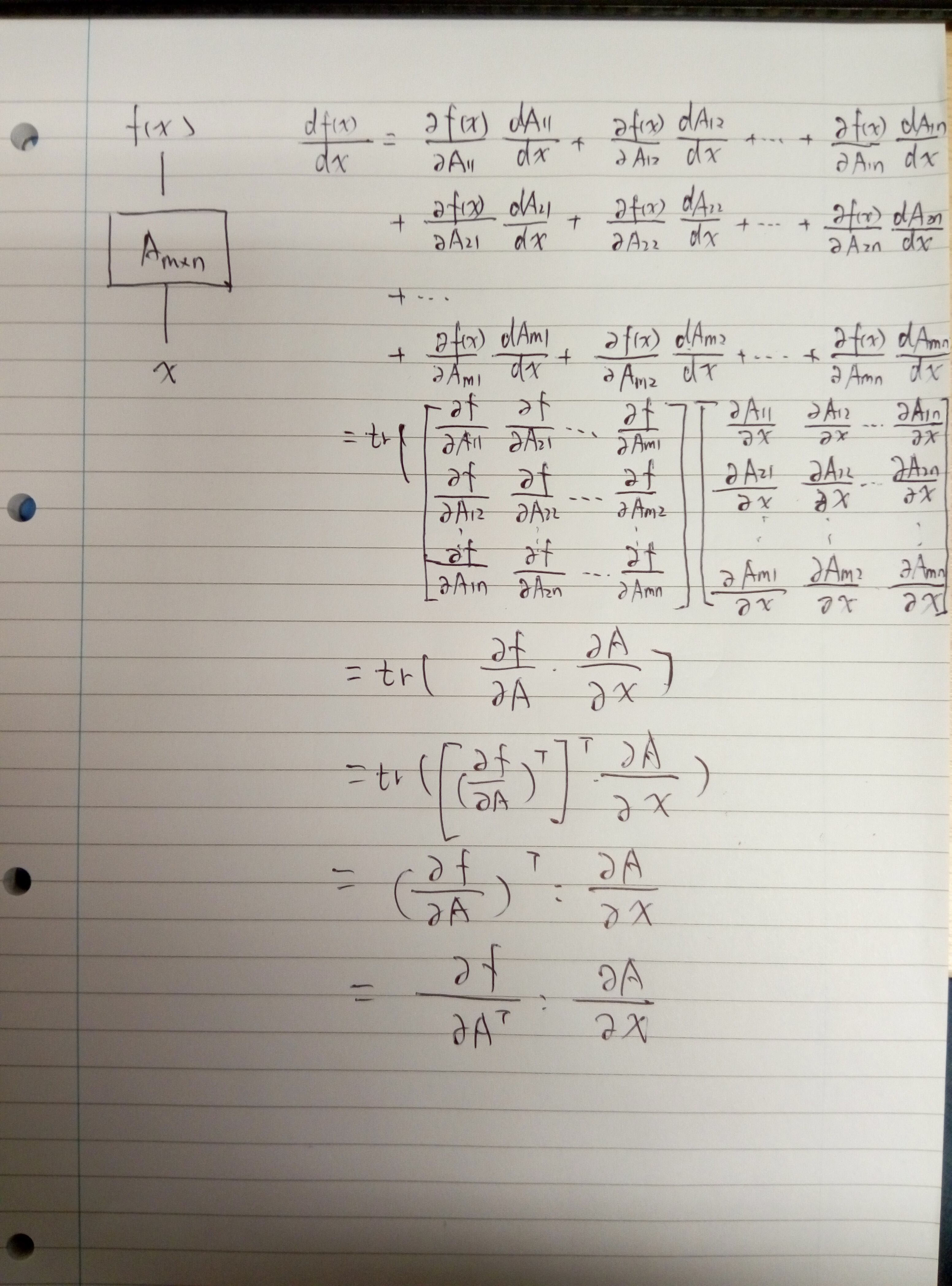
最后让我们看个例子,f(x)为x的函数,f(x)和x都为标量,但是中间有个$A_{m*n}$的矩阵作为他们的连接关系,求$\frac{df(x)}{dx}$

后来参照了一本介绍tensor的书

tensor.pdf

在30页提到了 $\cdot\cdot$运算符

我想我们这里可以表示成

$$\frac{df(x)}{dx}=\frac{\partial f(x)}{\partial A}\cdot\cdot\frac{\partial A}{\partial x}$$

这里说下我自己对$\cdot\cdot$运算符的理解

$$\mathbf{A}\cdot\cdot \mathbf{B} = \mathrm{tr}(\mathbf{A} \mathbf{B})$$

24, Aug, 2018 update

$$\frac{df(x)}{dx}=\frac{\partial f(x)}{\partial A}:\frac{\partial A}{\partial x}$$

注意$\frac{\partial f(x)}{\partial A}$的尺寸与A的大小应该一致

$$\frac{d(\mathbf{A}:\mathbf{F(\mathbf X)})}{d\mathbf{X}} = \mathbf A \circ \frac{d\mathbf F(\mathbf X)}{d\mathbf X}$$