CogVideoX-5b及I2V详解（包含代码、论文详解）

1、概述

简介

CogVideoX是智谱开放平台中最新上线的视频模型，现已支持文生视频、图生视频多个能力，让用户可以在开放平台使用和调用视频模型能力，轻松高效地完成艺术视频创作。体验中心支持多种生成方式，包括文本生成视频、图片生成视频，可应用于广告制作、电影剪辑、短视频制作等领域。 

相关演示信息可查看github主页

历史版本信息

• 2022/5/19: 开源了 CogVideo 视频生成模型，这是首个开源的基于 Transformer 的大型文本生成视频模型，发表于 ICLR'23 论文 。
• 2024/8/6: 开源 CogVideoX 系列视频生成模型的第一个模型, CogVideoX-2B。
• 2024/8/27: 开源 CogVideoX 系列更大的模型 CogVideoX-5B 。
• 2024/9/19: 开源 CogVideoX 系列图生视频模型 CogVideoX-5B-I2V 。该模型可以将一张图像作为背景输入，结合提示词一起生成视频，具有更强的可控性。

本篇博客将主要介绍CogvideoX-5B、CogVideoX-5B-I2V的文生视频及图生视频的功能。

具体配置要求

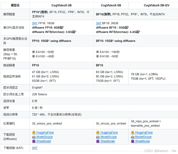
官方链接

体验平台：智谱清言

Github链接：https://github.com/THUDM/CogVideo

modelscope链接：魔搭社区（5b-I2V），魔搭社区（5b）

论文地址：https://arxiv.org/pdf/2408.06072

官方飞书文档：Docs

2、论文

这篇论文其实并没有提供太多的信息，个人建议想要学习的朋友还是着眼于代码，论文和代码同时理解。

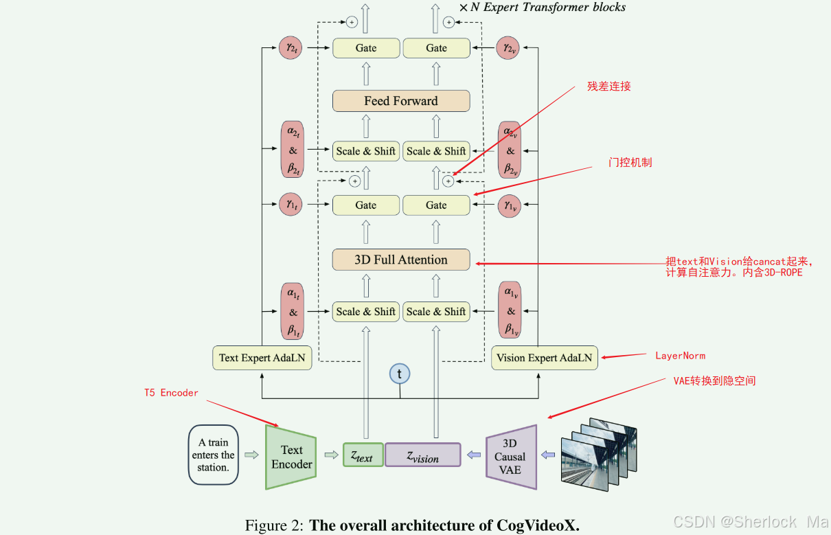
整体其实是diffusion结构，不过论文中没有提，论文中提到的整体架构其实是Diffusion的去噪模型，也就是使用VAE+Transformer进行去噪处理。

去噪模块

Transformer的整体架构如下，和其他的Transformer没有太大区别，主要增加了Gate（门控机制），将attention替换为3D Full Attention，并加入了3D-ROPE，虽然看起来是新东西，解析代码可知，这个attention其实是将text和Vision的隐空间concat起来，然后计算多头自注意力。

VAE

图3a所展示的VAE（变分自编码器）架构图，为我们揭示了CogVideoX模型中视频数据压缩与重建的核心机制。这一过程涉及到精心设计的上采样（upsampling）和下采样（downsampling）步骤，它们都是基于ResNet架构的改进版本，以适应视频数据的三维特性。

下采样过程（Encoder）

1. 视频压缩：Encoder的职责是将输入的视频数据从原始的高分辨率和高帧率压缩到更低的维度。具体来说，它将视频的空间维度从压缩到，时间维度从4f+1压缩到f。这一压缩比例大约是4×8×8=256倍，有效地减少了数据量，为后续的处理降低了计算成本。

2. 转换到隐空间：压缩后的视频数据被进一步转换到一个隐空间，这个空间捕获了视频的潜在特征。在这个空间中，视频数据被编码为一个潜在表示，这个表示将用于控制视频的生成过程。

上采样过程（Decoder）

1. 视频重建：在视频生成的最后阶段，Decoder负责将隐空间中的潜在表示还原回原始的视频空间。它通过上采样过程逐步恢复视频的空间和时间维度，最终生成与输入视频具有相同分辨率和帧率的视频。

2. 细节恢复：Decoder的设计确保了在重建过程中，视频的细节和动态变化得以保留。通过精心设计的网络结构，Decoder能够从潜在表示中恢复出丰富的视觉内容，包括颜色、纹理、运动等。

论文中f+1的1为什么要单独编码？

作者回复的答案：因为这个vae模型是从图像的vae迁移过来的，所有图像的vae不适合直接压视频。如果我们把这个1单独编码，其实相当于把第一帧重复成4帧，这样做编码，这样就可以尽可能保留vae原来的预训练能力，也保留第一帧中的视频内容，换句话说，压缩的效果更好。

我的理解：

• VAE最初是为图像设计的，它能够将图像数据压缩到一个潜在空间，并从这个空间重建图像。图像是二维数据，只有空间信息（高度和宽度）。直接将图像VAE应用于视频会导致不匹配，因为视频包含时间维度上的变化。
• 单独编码这一额外帧的原因是，这样做可以模拟视频的时间连续性，即使VAE模型原本是为处理图像设计的。通过这种方式，模型能够更好地处理视频数据，同时保留其在图像上预训练的能力。
• 将第一帧重复成四帧，意味着在时间维度上复制第一帧，从而在VAE的潜在空间中为视频建立一个起点。这样做可以帮助模型在生成视频时保持第一帧的内容和特征，这对于视频的连贯性和质量至关重要。

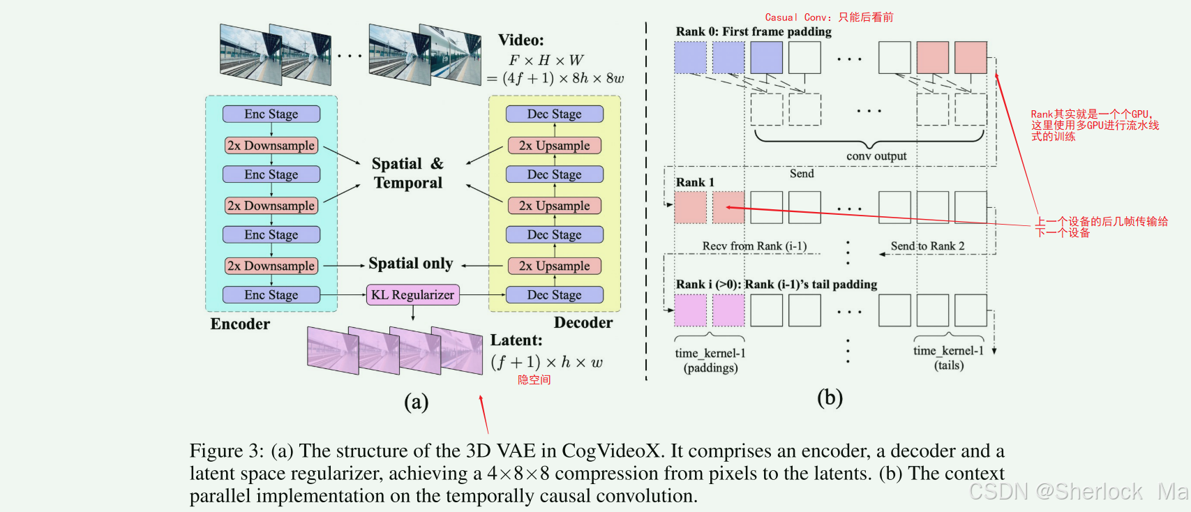
因果卷积（Casual Conv）

图3b展示的是因果卷积，即在每个时间步，因果卷积只考虑当前和之前的帧，而不包括未来的帧。这可以通过在卷积操作中使用特定的填充（padding）策略来实现，确保未来信息不会“泄露”到当前的预测中。

多GPU流水线式运行

图3b展示了这部分内容。具体来说，在训练过程中将这些视频分割为很多段，每段分配到多个处理单元（如GPU）。每个处理单元（或称为rank）处理一个数据段，并且只将其处理结果的最后几帧发送给下一个处理单元。

所有单元并行运行，以流水线的形式运作，即GPU0处理第1个片段，处理完后把最后几帧传给GPU1，GPU1开始处理第2个片段，同时GPU0开始处理第k个片段。

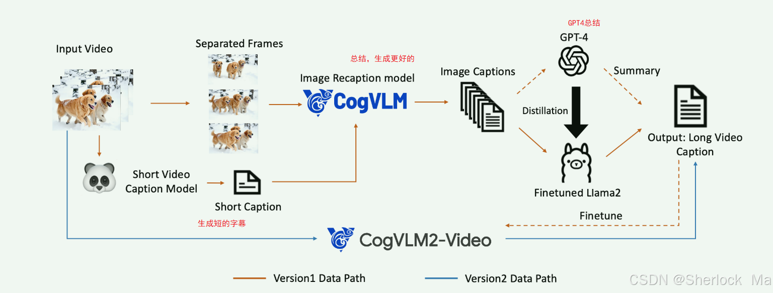
数据收集：

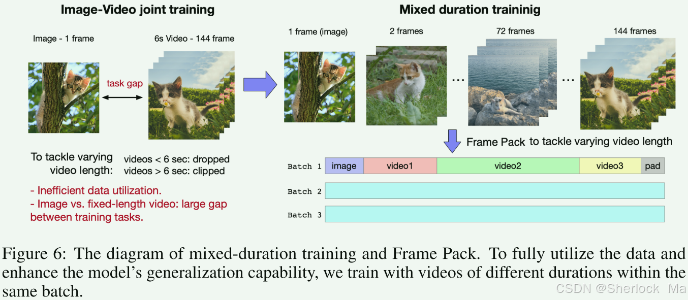
Frame Pack

在标准的深度学习训练中，一个批次内的所有样本通常需要具有相同的形状，以便于并行处理。然而，视频数据通常由不同长度的帧序列组成，这导致了直接处理上的困难。

为了解决这个问题，Frame Pack技术通过将不同长度的视频帧序列填充到相同的长度，使得它们可以被一起处理。具体来说，它通过创建一个虚拟的批次，其中每个视频帧序列都被填充或截断到一个预定的最大长度（图像算1帧视频）。这样，即使原始视频帧数不同，经过Frame Pack处理后，它们在每个批次中都具有相同的维度，从而可以被模型并行处理。

3、代码

环境配置

下载权重及代码，注意检查是不是下全了，尤其是权重。

git clone https://github.com/THUDM/CogVideo
git clone https://modelscope.cn/models/ZhipuAI/CogVideoX-5b

把项目文件放在一起，权重位置决定下文的model_path怎么写，列如我是这样的，我的model_path就是CogVideoX-5b

conda新建环境，注意必须是Python3.10-3.12的版本，torch版本为2.4

然后安装所需库

pip install -r requirements.txt

注意需要保证diffusers库的版本，要随着版本不断更新，目前已经更新到0.30.3，如果发布0.31.0，还需要继续更新。

pip install diffusers==0.30.3

代码讲解

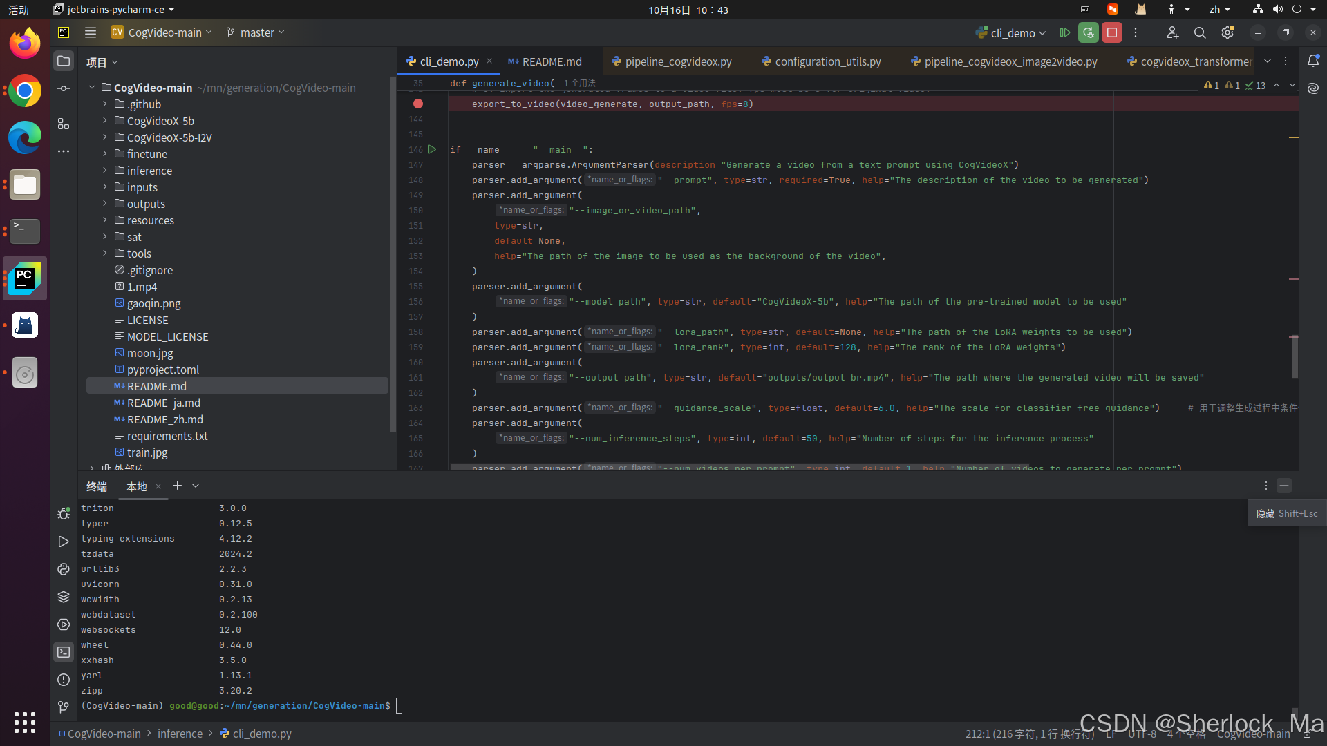
作者提供了一个演示文件cli_demo.py，所有操作通过diffusers库调用。

cli_demo.py

具体来说，这个代码提供了如下的参数供用户调节。

parser.add_argument("--prompt", type=str, required=True, help="The description of the video to be generated")
parser.add_argument(
        "--image_or_video_path",
        type=str,
        default=None,
        help="The path of the image to be used as the background of the video",
    )
parser.add_argument(
        "--model_path", type=str, default="CogVideoX-5b", help="The path of the pre-trained model to be used"
    )
parser.add_argument("--lora_path", type=str, default=None, help="The path of the LoRA weights to be used")
parser.add_argument("--lora_rank", type=int, default=128, help="The rank of the LoRA weights")
parser.add_argument(
        "--output_path", type=str, default="outputs/output_br.mp4", help="The path where the generated video will be saved"
    )
parser.add_argument("--guidance_scale", type=float, default=6.0, help="The scale for classifier-free guidance")     # 用于调整生成过程中条件信息（如文本描述）对生成结果的影响程度。
parser.add_argument(
        "--num_inference_steps", type=int, default=50, help="Number of steps for the inference process"
    )
parser.add_argument("--num_videos_per_prompt", type=int, default=1, help="Number of videos to generate per prompt")
parser.add_argument(
        "--generate_type", type=str, default="t2v", help="The type of video generation (e.g., 't2v', 'i2v', 'v2v')"
    )
parser.add_argument(
        "--dtype", type=str, default="bfloat16", help="The data type for computation (e.g., 'float16' or 'bfloat16')"
    )
parser.add_argument("--seed", type=int, default=42, help="The seed for reproducibility")

我们常用的有：

• prompt：提示词，生成视频的文本提示
• image_or_video_path：视频或图像的地址，用于I2V或V2V模式，一定要把下面的generate_type同步改了
• model_path：模型权重文件的地址，需要自己指定本地的，否则会到hugging face下载
• output_path：生成视频的存放位置
• num_inference_steps：推理步骤，一般越长约好
• generate_type：模式，默认t2v，即文生视频；还有i2v和v2v，即图生视频和视频续写

我们可以使用如下参数，快速启动代码。

注意：我是通过pycharm右上角的编辑配置运行的，习惯命令行的记得加上python cli_demo.py

--prompt
"The Glenfinnan Viaduct is a historic railway bridge.It is a stunning sight as a steam train leaves the bridge, traveling over the arch-covered viaduct. The landscape is dotted with lush greenery and rocky mountains"
--model_path
CogVideoX-5b

传入参数后，代码会在178行进入在35行定义的函数 generate_video。

以t2v为例，然后经过初始化后，来到120行，进入diffusers开始运行模型。

    elif generate_type == "t2v":
        video_generate = pipe(
            prompt=prompt,
            height=480,
            width=720,
            num_videos_per_prompt=num_videos_per_prompt,
            num_inference_steps=num_inference_steps,
            num_frames=49,
            use_dynamic_cfg=True,
            guidance_scale=guidance_scale,
            generator=torch.Generator().manual_seed(seed),      # 这些数对于每次使用相同的种子值时都是相同的。
        ).frames[0]     #　PIL,49帧

模型运行完成，会运行到143行，进入视频生成环节，即将diffusion运行的结果转化为真正的视频。然后保存并输出。

# 5. Export the generated frames to a video file. fps must be 8 for original video.
export_to_video(video_generate, output_path, fps=8)

pipeline_cogvideox.py

整个模型的核心代码，代码会进入596行开始运行，作者的代码逻辑和注释非常清晰，总体上分为8个部分，前2个部分为检查和设置参数，故不多介绍。

        # 1. Check inputs. Raise error if not correct
        self.check_inputs(
            prompt,
            height,
            width,
            negative_prompt,
            callback_on_step_end_tensor_inputs,
            prompt_embeds,
            negative_prompt_embeds,
        )
        self._guidance_scale = guidance_scale
        self._interrupt = False

        # 2. Default call parameters
        if prompt is not None and isinstance(prompt, str):
            batch_size = 1
        elif prompt is not None and isinstance(prompt, list):
            batch_size = len(prompt)
        else:
            batch_size = prompt_embeds.shape[0]

        device = self._execution_device

        # here `guidance_scale` is defined analog to the guidance weight `w` of equation (2) 用于调整生成过程中条件信息（如文本描述）对生成结果的影响程度。
        # of the Imagen paper: https://arxiv.org/pdf/2205.11487.pdf . `guidance_scale = 1`
        # corresponds to doing no classifier free guidance.
        do_classifier_free_guidance = guidance_scale > 1.0

第3个部分是对prompt的编码部分，这个部分的代码是将两个prompt（正向和反向，即想要出现什么和不想要出现什么）转换为长度为226,channel为4096的两个向量。使用的模型是T5的Encoder部分。

prompt_embeds, negative_prompt_embeds = self.encode_prompt(     # 最后的输出：两个都是[batch_size,max_sequence_len,4096]=[1,226,4096]
      prompt,         # 正提示词，即想要的
      negative_prompt,    # 反向提示词，即不想要的东西，我这里没设置
      do_classifier_free_guidance,
      num_videos_per_prompt=num_videos_per_prompt, # 每个prompt几个视频，这里为1
      prompt_embeds=prompt_embeds,  # None
      negative_prompt_embeds=negative_prompt_embeds,   # None
      max_sequence_length=max_sequence_length,  # 226，序列最大长度，不够补齐，多了截断
            device=device,
        )
if do_classifier_free_guidance:
      prompt_embeds = torch.cat([negative_prompt_embeds, prompt_embeds], dim=0)   # [2b,max_sequence_len,4096]=[2,226,4096]

模型架构：

T5EncoderModel(
  (shared): Embedding(32128, 4096)
  (encoder): T5Stack(
    (embed_tokens): Embedding(32128, 4096)
    (block): ModuleList(
      (0): T5Block(
        (layer): ModuleList(
          (0): T5LayerSelfAttention(
            (SelfAttention): T5Attention(
              (q): Linear(in_features=4096, out_features=4096, bias=False)
              (k): Linear(in_features=4096, out_features=4096, bias=False)
              (v): Linear(in_features=4096, out_features=4096, bias=False)
              (o): Linear(in_features=4096, out_features=4096, bias=False)
              (relative_attention_bias): Embedding(32, 64)
            )
            (layer_norm): T5LayerNorm()
            (dropout): Dropout(p=0.1, inplace=False)
          )
          (1): T5LayerFF(
            (DenseReluDense): T5DenseGatedActDense(
              (wi_0): Linear(in_features=4096, out_features=10240, bias=False)
              (wi_1): Linear(in_features=4096, out_features=10240, bias=False)
              (wo): Linear(in_features=10240, out_features=4096, bias=False)
              (dropout): Dropout(p=0.1, inplace=False)
              (act): NewGELUActivation()
            )
            (layer_norm): T5LayerNorm()
            (dropout): Dropout(p=0.1, inplace=False)
          )
        )
      )
      (1-23): 23 x T5Block(
        (layer): ModuleList(
          (0): T5LayerSelfAttention(
            (SelfAttention): T5Attention(
              (q): Linear(in_features=4096, out_features=4096, bias=False)
              (k): Linear(in_features=4096, out_features=4096, bias=False)
              (v): Linear(in_features=4096, out_features=4096, bias=False)
              (o): Linear(in_features=4096, out_features=4096, bias=False)
            )
            (layer_norm): T5LayerNorm()
            (dropout): Dropout(p=0.1, inplace=False)
          )
          (1): T5LayerFF(
            (DenseReluDense): T5DenseGatedActDense(
              (wi_0): Linear(in_features=4096, out_features=10240, bias=False)
              (wi_1): Linear(in_features=4096, out_features=10240, bias=False)
              (wo): Linear(in_features=10240, out_features=4096, bias=False)
              (dropout): Dropout(p=0.1, inplace=False)
              (act): NewGELUActivation()
            )
            (layer_norm): T5LayerNorm()
            (dropout): Dropout(p=0.1, inplace=False)
          )
        )
      )
    )
    (final_layer_norm): T5LayerNorm()
    (dropout): Dropout(p=0.1, inplace=False)
  )
)

具体而言，代码会跳入encode_prompt()里，主要的代码在292行和316行，分别是对prompt和negative_prompt的处理，两个部分完全一样，所以本文只讲1个。

if prompt_embeds is None:
    prompt_embeds = self._get_t5_prompt_embeds(     # [b,max_sequence_len,4096]=[1,226,4096]
        prompt=prompt,
        num_videos_per_prompt=num_videos_per_prompt,
        max_sequence_length=max_sequence_length,
        device=device,
        dtype=dtype,
    )

代码会进一步跳入_get_t5_prompt_embeds()，其中tokenizer在217行，主要将prompt切成token，并转换为token id；encoder在235行，主要将token id转换为向量。

text_inputs = self.tokenizer(   # 里面包括两个，attn_mask和input_ids都是[b,max_sequence_len]=[1,226]
    prompt,
    padding="max_length",
    max_length=max_sequence_length,     # 长度超过max_length，则将执行截断，
    truncation=True,        # 执行截断
    add_special_tokens=True,
    return_tensors="pt",    # 表示tokenizer的输出将以PyTorch张量的形式返回
)
text_input_ids = text_inputs.input_ids  # 只取出input_ids，即tokenizer切分的token id

tokenizer输出的是[1,226]的向量，而text_encoder将其embedding为[1,226,4096]的向量。

prompt_embeds = self.text_encoder(text_input_ids.to(device))[0]     # [b,max_sequence_len,4096]=[1,226,4096]
prompt_embeds = prompt_embeds.to(dtype=dtype, device=device)

需要注意的是，在主代码部分，还会将prompt和negative_prompt的处理结果在第0维合并，即[2,226,4096]。

第4个部分是对时间维度的处理

# 4. Prepare timesteps
timesteps, num_inference_steps = retrieve_timesteps(self.scheduler, num_inference_steps, device, timesteps)     # [1000]=[999,...,0]  1000
self._num_timesteps = len(timesteps)

这个部分实际上是把时间步切分为num_inference_steps个，如我设置的是50,那就会把1000划分为50个部分：

tensor([999, 979, 959, 939, 919, 899, 879, 859, 839, 819, 799, 779, 759, 739,
        719, 699, 679, 659, 639, 619, 599, 579, ..., 399, 379, 359, 339, 319, 299, 279, 259, 239, 219, 199, 179,
        159, 139, 119,  99,  79,  59,  39,  19], device='cuda:0')

第5个部分，即初始化潜在空间。总体上就是初始化一个符合正态分布的噪声，满足尺寸为[b,frame+1,latent channel,h,w]=[1,13,16,60,90]，实际上就是论文中的对帧率进行4倍下采样，对宽高进行8倍下采样的结果。

# 5. Prepare latents.
latent_channels = self.transformer.config.in_channels       # 16
latents = self.prepare_latents(         # 生成的[b,frame+1,latent channel,h,w]=[1,13,16,60,90]
    batch_size * num_videos_per_prompt,
    latent_channels,
    num_frames,
    height,
    width,
    prompt_embeds.dtype,
    device,
    generator,
    latents,   # None
)

核心代码在342行：

if latents is None:
    latents = randn_tensor(shape, generator=generator, device=device, dtype=dtype)      # [b,f+1,num_channels_latents,h,w]=[1,13,16,60,90]

第6部分主要是设置参数，故不多介绍

第7部分是生成3D-ROPE编码，简单来说，就是用来生成cos和sin的位置编码，长度均为[17550,64]

# 7. Create rotary embeds if required       # 3D-ROPE
image_rotary_emb = (
    self._prepare_rotary_positional_embeddings(height, width, latents.size(1), device)
    if self.transformer.config.use_rotary_positional_embeddings
    else None
)       # 里面有两个，分别是cos和sin的，长度均为[17550,64]

代码会跳转到441行，

def _prepare_rotary_positional_embeddings(
    self,
    height: int,
    width: int,
    num_frames: int,
    device: torch.device,
) -> Tuple[torch.Tensor, torch.Tensor]:
    grid_height = height // (self.vae_scale_factor_spatial * self.transformer.config.patch_size)   # 30
    grid_width = width // (self.vae_scale_factor_spatial * self.transformer.config.patch_size)     # 45
    base_size_width = 720 // (self.vae_scale_factor_spatial * self.transformer.config.patch_size)  # 45
    base_size_height = 480 // (self.vae_scale_factor_spatial * self.transformer.config.patch_size) # 30

    grid_crops_coords = get_resize_crop_region_for_grid(   # ((0,0),(30,45))
        (grid_height, grid_width), base_size_width, base_size_height
    )
    freqs_cos, freqs_sin = get_3d_rotary_pos_embed(   # 计算每个网格的位置编码
        embed_dim=self.transformer.config.attention_head_dim,
        crops_coords=grid_crops_coords,
        grid_size=(grid_height, grid_width),
        temporal_size=num_frames,
        use_real=True,
    )       # [17550,64]

    freqs_cos = freqs_cos.to(device=device)   # 计算cos
    freqs_sin = freqs_sin.to(device=device)   # 计算sin
    return freqs_cos, freqs_sin

get_3d_rotary_pos_embed()是核心部分，接下来，我们来看一下。

    start, stop = crops_coords
    grid_h = np.linspace(start[0], stop[0], grid_size[0], endpoint=False, dtype=np.float32)
    grid_w = np.linspace(start[1], stop[1], grid_size[1], endpoint=False, dtype=np.float32)
    grid_t = np.linspace(0, temporal_size, temporal_size, endpoint=False, dtype=np.float32)

    # Compute dimensions for each axis
    dim_t = embed_dim // 4
    dim_h = embed_dim // 8 * 3
    dim_w = embed_dim // 8 * 3

    # Temporal frequencies
    freqs_t = 1.0 / (theta ** (torch.arange(0, dim_t, 2).float() / dim_t))  # [8]
    grid_t = torch.from_numpy(grid_t).float()   # [13]
    freqs_t = torch.einsum("n , f -> n f", grid_t, freqs_t)     # [13,8]
    freqs_t = freqs_t.repeat_interleave(2, dim=-1)      # [13,16]将频率网格在最后一个维度上重复两倍。

    # Spatial frequencies for height and width
    freqs_h = 1.0 / (theta ** (torch.arange(0, dim_h, 2).float() / dim_h))  # [12]
    freqs_w = 1.0 / (theta ** (torch.arange(0, dim_w, 2).float() / dim_w))
    grid_h = torch.from_numpy(grid_h).float()   # [30]
    grid_w = torch.from_numpy(grid_w).float()
    freqs_h = torch.einsum("n , f -> n f", grid_h, freqs_h) # [30,12]
    freqs_w = torch.einsum("n , f -> n f", grid_w, freqs_w)
    freqs_h = freqs_h.repeat_interleave(2, dim=-1)      # [30,24]
    freqs_w = freqs_w.repeat_interleave(2, dim=-1)

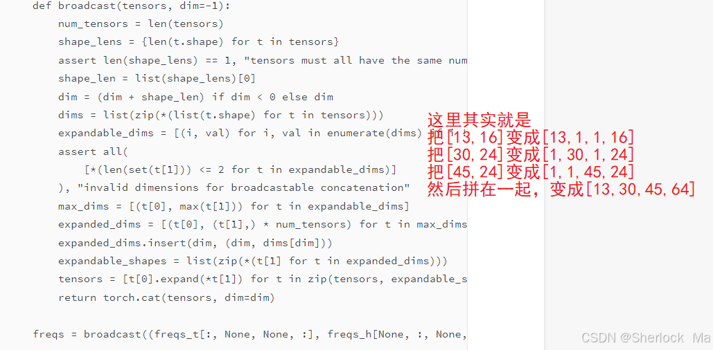
    # Broadcast and concatenate tensors along specified dimension
    def broadcast(tensors, dim=-1):
        num_tensors = len(tensors)
        shape_lens = {len(t.shape) for t in tensors}
        assert len(shape_lens) == 1, "tensors must all have the same number of dimensions"
        shape_len = list(shape_lens)[0]
        dim = (dim + shape_len) if dim < 0 else dim
        dims = list(zip(*(list(t.shape) for t in tensors)))
        expandable_dims = [(i, val) for i, val in enumerate(dims) if i != dim]
        assert all(
            [*(len(set(t[1])) <= 2 for t in expandable_dims)]
        ), "invalid dimensions for broadcastable concatenation"
        max_dims = [(t[0], max(t[1])) for t in expandable_dims]
        expanded_dims = [(t[0], (t[1],) * num_tensors) for t in max_dims]
        expanded_dims.insert(dim, (dim, dims[dim]))
        expandable_shapes = list(zip(*(t[1] for t in expanded_dims)))
        tensors = [t[0].expand(*t[1]) for t in zip(tensors, expandable_shapes)]
        return torch.cat(tensors, dim=dim)

    freqs = broadcast((freqs_t[:, None, None, :], freqs_h[None, :, None, :], freqs_w[None, None, :, :]), dim=-1)    # [13,30,45,64]

    t, h, w, d = freqs.shape
    freqs = freqs.view(t * h * w, d)        # [17550,64]

    # Generate sine and cosine components
    sin = freqs.sin()
    cos = freqs.cos()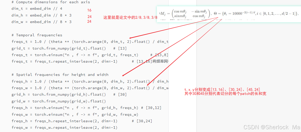

第8个部分是整个代码的核心部分，这个部分主要是使用定义的Transformer模型进行去噪，直到生成图像。

第8部分的核心逻辑就是diffusion的去噪过程包括了利用去噪器预测噪声和利用预测结果生成新的潜在空间，其中第682行是transformer模型作为去噪器，预测噪声：

# predict noise model_output
noise_pred = self.transformer(      # 把transformer架构当做去噪器，进行去噪
    hidden_states=latent_model_input,
    encoder_hidden_states=prompt_embeds,
    timestep=timestep,
    image_rotary_emb=image_rotary_emb,
    return_dict=False,
)[0]        # 输出：[2b,f+1,latent channel,h,w]=[2,13,16,60,90]
noise_pred = noise_pred.float()

第704行是使用去噪结果生成新的潜在空间

else:
    latents, old_pred_original_sample = self.scheduler.step(    # 根据预测的噪声和当前时间步，使用 self.scheduler.step计算前一个噪声样本。
        noise_pred,
        old_pred_original_sample,
        t,
        timesteps[i - 1] if i > 0 else None,
        latents,
        **extra_step_kwargs,
        return_dict=False,
    )

我们先来看transformer的forward过程：

这个过程中，首先先将时间t embedding为[2b,c]=[2,512]的向量，然后将文本向量和隐空间噪声一起进行embedding，变成[2b,text_seq_length,c]=[2,17726,3072]的向量，然后再分别拆回文本的向量和视频向量。第三步进入transformer模块进行计算。

• 其中17726=226+17750,17750=13*45*30(f+1*w*h)，也就是将每个画面切分为45*30的patch，为后面的计算做准备。

# 1. Time embedding
timesteps = timestep
t_emb = self.time_proj(timesteps)   # [2,3072]

# timesteps does not contain any weights and will always return f32 tensors
# but time_embedding might actually be running in fp16. so we need to cast here.
# there might be better ways to encapsulate this.
t_emb = t_emb.to(dtype=hidden_states.dtype)
emb = self.time_embedding(t_emb, timestep_cond)     # [2,512]

# 2. Patch embedding
hidden_states = self.patch_embed(encoder_hidden_states, hidden_states)
hidden_states = self.embedding_dropout(hidden_states)   # [2b,text_seq_length,c][2,17726,3072]

text_seq_length = encoder_hidden_states.shape[1]    # 226
encoder_hidden_states = hidden_states[:, :text_seq_length]
hidden_states = hidden_states[:, text_seq_length:]

# 3. Transformer blocks
for i, block in enumerate(self.transformer_blocks):
    if self.training and self.gradient_checkpointing:

        def create_custom_forward(module):
            def custom_forward(*inputs):
                return module(*inputs)

            return custom_forward

        ckpt_kwargs: Dict[str, Any] = {"use_reentrant": False} if is_torch_version(">=", "1.11.0") else {}
        hidden_states, encoder_hidden_states = torch.utils.checkpoint.checkpoint(
            create_custom_forward(block),
            hidden_states,
            encoder_hidden_states,
            emb,
            image_rotary_emb,
            **ckpt_kwargs,
        )
    else:
        hidden_states, encoder_hidden_states = block(       # [2,17550,3072]，[2,226,3072]
            hidden_states=hidden_states,        # [2,17550,3072]
            encoder_hidden_states=encoder_hidden_states,    # [2,226,3072]
            temb=emb,
            image_rotary_emb=image_rotary_emb,
        )

transformer每个模块架构如下所示：

实际上可以看到，整个架构和普通的transformer差别不大，主要的差别在于多了门控机制(gate)和新的3D-Full-Attention

text_seq_length = encoder_hidden_states.size(1)

# norm & modulate
norm_hidden_states, norm_encoder_hidden_states, gate_msa, enc_gate_msa = self.norm1(
    hidden_states, encoder_hidden_states, temb
)

# attention
attn_hidden_states, attn_encoder_hidden_states = self.attn1(
    hidden_states=norm_hidden_states,
    encoder_hidden_states=norm_encoder_hidden_states,
    image_rotary_emb=image_rotary_emb,
)

hidden_states = hidden_states + gate_msa * attn_hidden_states
encoder_hidden_states = encoder_hidden_states + enc_gate_msa * attn_encoder_hidden_states

# norm & modulate
norm_hidden_states, norm_encoder_hidden_states, gate_ff, enc_gate_ff = self.norm2(
    hidden_states, encoder_hidden_states, temb
)

# feed-forward
norm_hidden_states = torch.cat([norm_encoder_hidden_states, norm_hidden_states], dim=1)
ff_output = self.ff(norm_hidden_states)

hidden_states = hidden_states + gate_ff * ff_output[:, text_seq_length:]
encoder_hidden_states = encoder_hidden_states + enc_gate_ff * ff_output[:, :text_seq_length]

return hidden_states, encoder_hidden_states

接下来来看一下attention部分，其实就是基本的multi-head attention，只不过为视觉部分增加了上述3D-ROPE

text_seq_length = encoder_hidden_states.size(1)

hidden_states = torch.cat([encoder_hidden_states, hidden_states], dim=1)    # 将文本和视频的向量拼接[2,17726,3072]

batch_size, sequence_length, _ = (
    hidden_states.shape if encoder_hidden_states is None else encoder_hidden_states.shape
)

if attention_mask is not None:
    attention_mask = attn.prepare_attention_mask(attention_mask, sequence_length, batch_size)
    attention_mask = attention_mask.view(batch_size, attn.heads, -1, attention_mask.shape[-1])

query = attn.to_q(hidden_states)    # Q
key = attn.to_k(hidden_states)      # K
value = attn.to_v(hidden_states)    # V

inner_dim = key.shape[-1]
head_dim = inner_dim // attn.heads  # 每个头处理64维数据

query = query.view(batch_size, -1, attn.heads, head_dim).transpose(1, 2)    # [2,48,17776,64]
key = key.view(batch_size, -1, attn.heads, head_dim).transpose(1, 2)
value = value.view(batch_size, -1, attn.heads, head_dim).transpose(1, 2)

if attn.norm_q is not None:
    query = attn.norm_q(query)
if attn.norm_k is not None:
    key = attn.norm_k(key)

# Apply RoPE if needed
if image_rotary_emb is not None:
    from .embeddings import apply_rotary_emb

    query[:, :, text_seq_length:] = apply_rotary_emb(query[:, :, text_seq_length:], image_rotary_emb)    # 仅在视频部分增加rope   
    if not attn.is_cross_attention:
        key[:, :, text_seq_length:] = apply_rotary_emb(key[:, :, text_seq_length:], image_rotary_emb)

hidden_states = F.scaled_dot_product_attention(     # 计算attention
    query, key, value, attn_mask=attention_mask, dropout_p=0.0, is_causal=False
)

hidden_states = hidden_states.transpose(1, 2).reshape(batch_size, -1, attn.heads * head_dim)

# linear proj
hidden_states = attn.to_out[0](hidden_states)
# dropout
hidden_states = attn.to_out[1](hidden_states)

encoder_hidden_states, hidden_states = hidden_states.split(     # 拆分
    [text_seq_length, hidden_states.size(1) - text_seq_length], dim=1
)
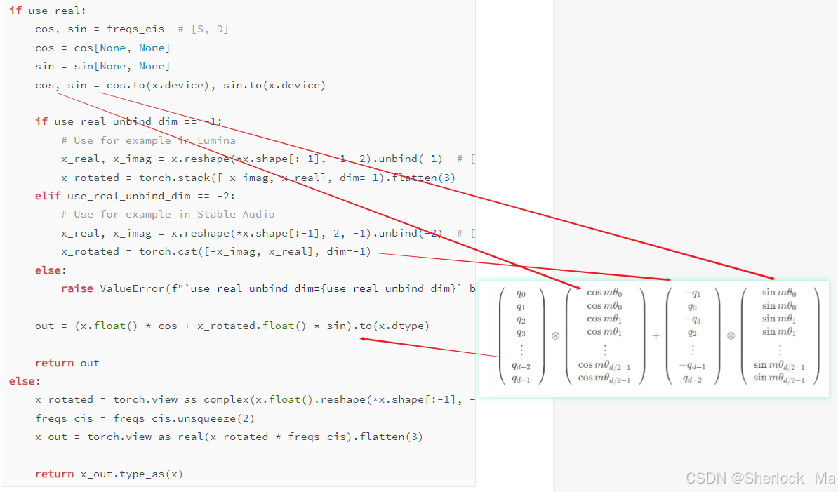
return hidden_states, encoder_hidden_states

其中的apply_rotary_emb是计算3D-ROPE的部分，具体运算过程可参考下图

再来看一下schduler.step的流程。建议读者先掌握diffusion的数学推理，再详细了解这一部分。简单来说，

1. 这部分代码首先计算的累乘，
2. 然后通过transformer预测的噪声和上一步的隐空间状态计算pred_original_sample，
3. 再引入新的噪声noise，这个噪声是从标准正态分布中采样的，用于在样本更新过程中引入随机性。
4. 再通过pred_original_sample和noise计算prev_sample，即最终的输出结果。

总结来说，这几行代码实现了扩散模型中的一个关键步骤，即通过结合当前样本、预测的原始样本和噪声来生成前一时间步的样本。这个过程涉及到计算中间变量、生成噪声，并使用这些组件来更新样本。

# Notation (<variable name> -> <name in paper>
# - pred_noise_t -> e_theta(x_t, t)
# - pred_original_sample -> f_theta(x_t, t) or x_0
# - std_dev_t -> sigma_t
# - eta -> η
# - pred_sample_direction -> "direction pointing to x_t"
# - pred_prev_sample -> "x_t-1"

# 1. get previous step value (=t-1)
prev_timestep = timestep - self.config.num_train_timesteps // self.num_inference_steps

# 2. compute alphas, betas
alpha_prod_t = self.alphas_cumprod[timestep]    # 计算了当前时间步的α值的乘积
alpha_prod_t_prev = self.alphas_cumprod[prev_timestep] if prev_timestep >= 0 else self.final_alpha_cumprod  # 计算了前一时间步的α值的乘积
alpha_prod_t_back = self.alphas_cumprod[timestep_back] if timestep_back is not None else None

beta_prod_t = 1 - alpha_prod_t    # 计算了当前时间步的beta值的乘积

# 3. compute predicted original sample from predicted noise also called
# "predicted x_0" of formula (12) from https://arxiv.org/pdf/2010.02502.pdf
# To make style tests pass, commented out `pred_epsilon` as it is an unused variable
if self.config.prediction_type == "epsilon":
    pred_original_sample = (sample - beta_prod_t ** (0.5) * model_output) / alpha_prod_t ** (0.5)
    # pred_epsilon = model_output
elif self.config.prediction_type == "sample":
    pred_original_sample = model_output
    # pred_epsilon = (sample - alpha_prod_t ** (0.5) * pred_original_sample) / beta_prod_t ** (0.5)
elif self.config.prediction_type == "v_prediction":     # 推理走这里：计算预测的原始样本
    # 通过transformer预测的噪声和上一步的隐空间状态计算pred_original_sample
    pred_original_sample = (alpha_prod_t**0.5) * sample - (beta_prod_t**0.5) * model_output
    # pred_epsilon = (alpha_prod_t**0.5) * model_output + (beta_prod_t**0.5) * sample
else:
    raise ValueError(
        f"prediction_type given as {self.config.prediction_type} must be one of `epsilon`, `sample`, or"
        " `v_prediction`"
    )

h, r, lamb, lamb_next = self.get_variables(alpha_prod_t, alpha_prod_t_prev, alpha_prod_t_back)
mult = list(self.get_mult(h, r, alpha_prod_t, alpha_prod_t_prev, alpha_prod_t_back))
mult_noise = (1 - alpha_prod_t_prev) ** 0.5 * (1 - (-2 * h).exp()) ** 0.5   # 控制噪声的幅度，以确保样本的平滑过渡。

noise = randn_tensor(sample.shape, generator=generator, device=sample.device, dtype=sample.dtype)   # 在样本更新过程中引入随机性
prev_sample = mult[0] * sample - mult[1] * pred_original_sample + mult_noise * noise    # 结合了当前样本、预测的原始样本和噪声，以模拟从当前时间步到前一时间步的扩散过程。

if old_pred_original_sample is None or prev_timestep < 0:
    # Save a network evaluation if all noise levels are 0 or on the first step
    return prev_sample, pred_original_sample

直到所有扩散过程结束后，代码进入730行，使用VAE的decoder将潜在空间转换为视频数据，即将模型上采样回49*480*720的视频，然后将视频数据转换为PIL图像，输出。

if not output_type == "latent":
    video = self.decode_latents(latents)    # [b,c,f,h,w]=[1,3,49,480,720]
    video = self.video_processor.postprocess_video(video=video, output_type=output_type)    # PIL

至此，整个模型的大体流程就基本结束了。

然后代码会回到cli_demo执行export_to_video函数。其中的核心代码在180行，主要目的是将PIL图片写入文件，变成视频。

with imageio.get_writer(output_video_path, fps=fps) as writer:
    for frame in video_frames:
        writer.append_data(frame)

I2V部分

主要的区别如下：

首先在第5步，将image图像转换为[1,c,480,720]的图像，然后放入prepare_latents函数中生成潜在空间，因为只有一张照片，所以f=1，后面的12张为torch.zero生成的全0矩阵。最终latents和image_latents均为[1,13,16,60,90]

# 5. Prepare latents
image = self.video_processor.preprocess(image, height=height, width=width).to(      # [b,c,h,w]=[1,c,480,720]
    device, dtype=prompt_embeds.dtype
)

latent_channels = self.transformer.config.in_channels // 2
latents, image_latents = self.prepare_latents(      # [1,13,16,60,90]
    image,
    batch_size * num_videos_per_prompt,
    latent_channels,
    num_frames,
    height,
    width,
    prompt_embeds.dtype,
    device,
    generator,
    latents,
)

接着是第8步:

• 这里就是将latents和image_latents 在第三维(dim=2)concat到一起，最终的结果为[2,13,32,60,90]，注意在t2v模式，这里是[2,13,16,60,90]，也就是将两个16拼在一起了。
• 接着把新的latent_model_input输入到模型，进行预测。

latent_model_input = torch.cat([latents] * 2) if do_classifier_free_guidance else latents
latent_model_input = self.scheduler.scale_model_input(latent_model_input, t)

latent_image_input = torch.cat([image_latents] * 2) if do_classifier_free_guidance else image_latents
latent_model_input = torch.cat([latent_model_input, latent_image_input], dim=2)     # [2,13,32,60,90]

4.测试

The Glenfinnan Viaduct is a historic railway bridge.It is a stunning sight as a steam train leaves the bridge, traveling over the arch-covered viaduct. The landscape is dotted with lush greenery and rocky mountains

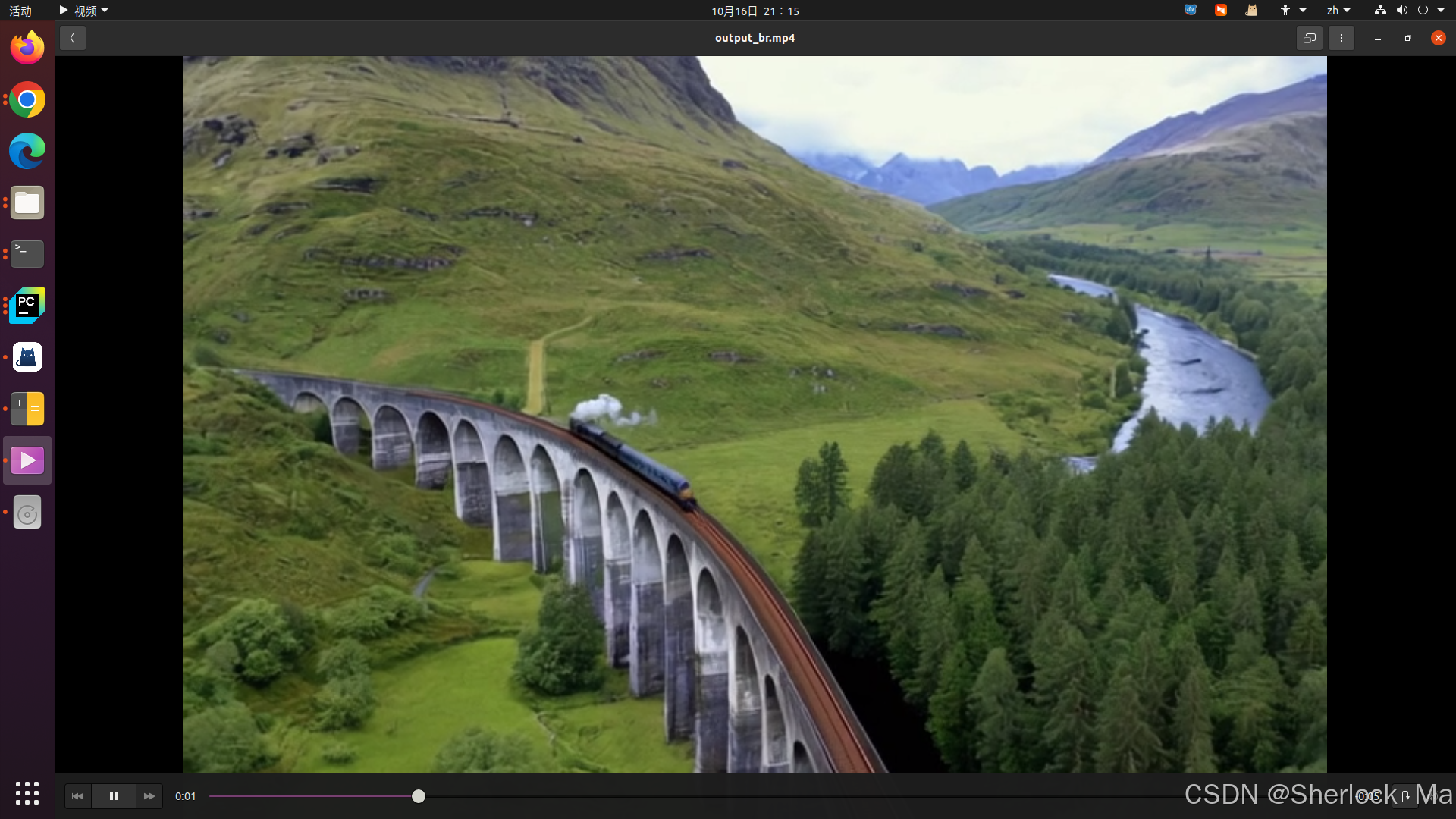
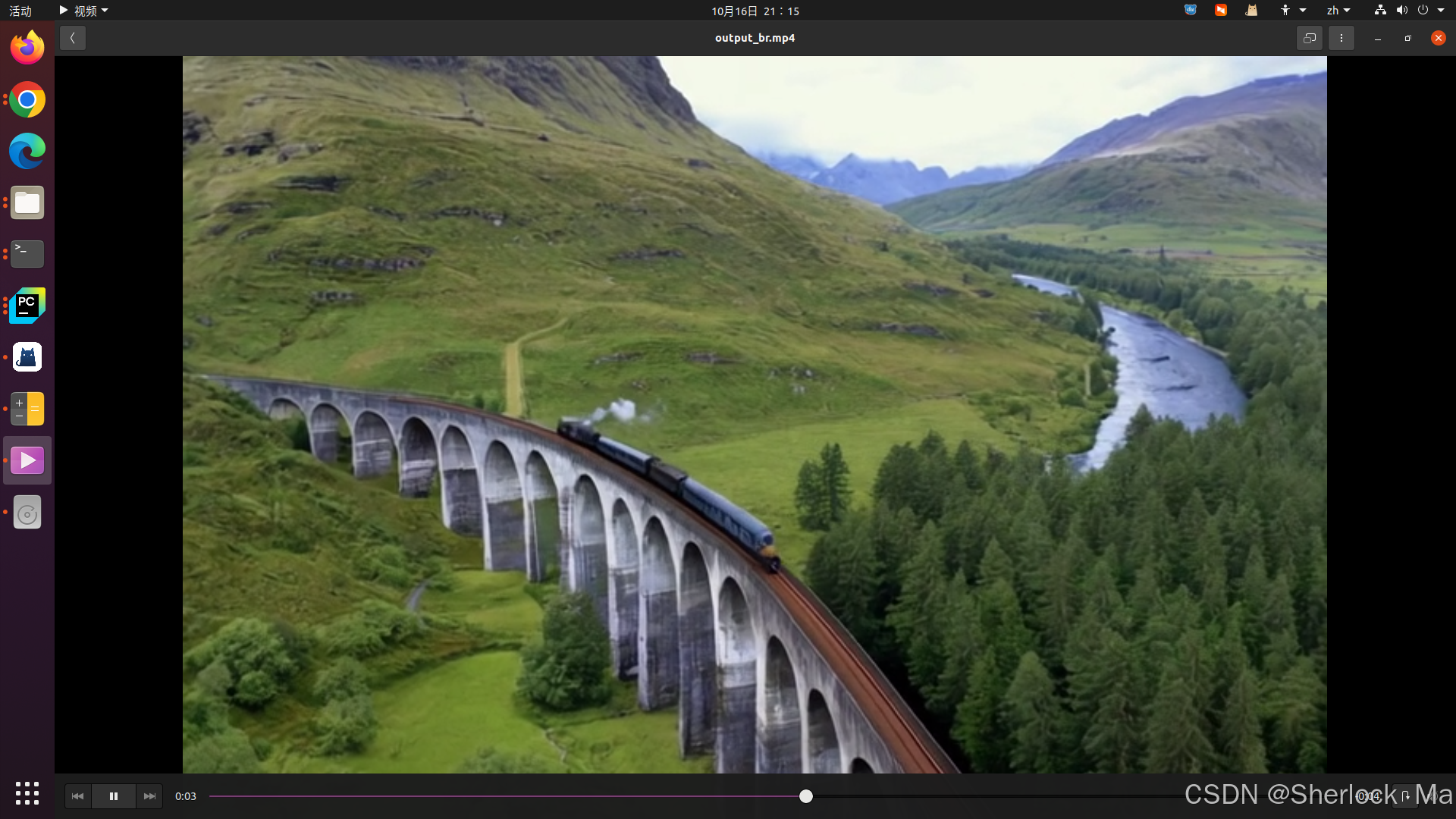
在对CogVideoX模型的输出进行观察时，我们注意到它在处理移动物体的场景时还存在一些挑战。例如，在生成的视频中，火车似乎突兀地从画面中凭空出现，并且其长度在在不断变长，更有趣的是，这种变长的方向与火车头部的行进方向相反。这一现象揭示了模型在捕捉和再现物体运动连贯性方面的潜力和需要改进的空间。

Don't move the position of the camera, the train is moving quickly along the track, the girl's long hair and skirt are blowing in the wind, the clouds are slowly moving and the sky is slowly getting darker.

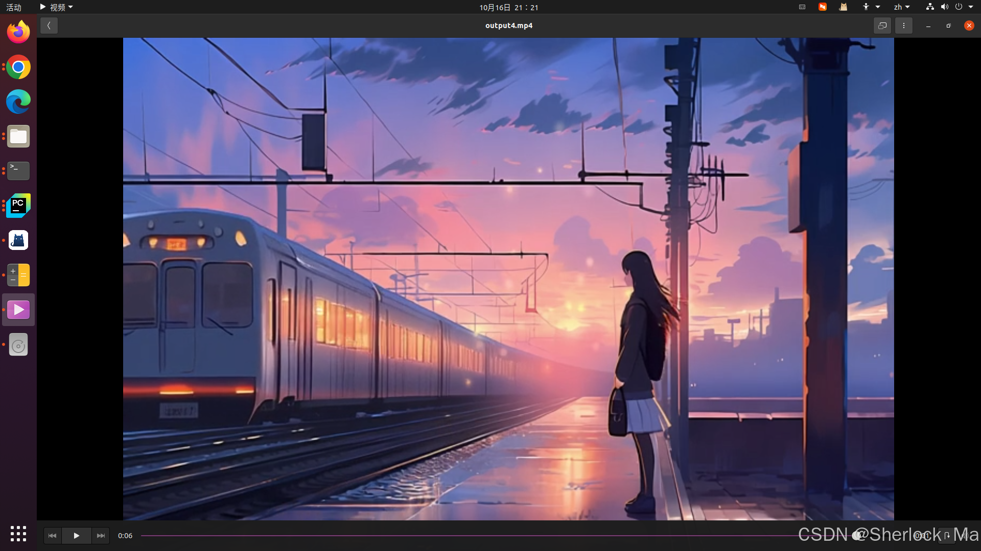
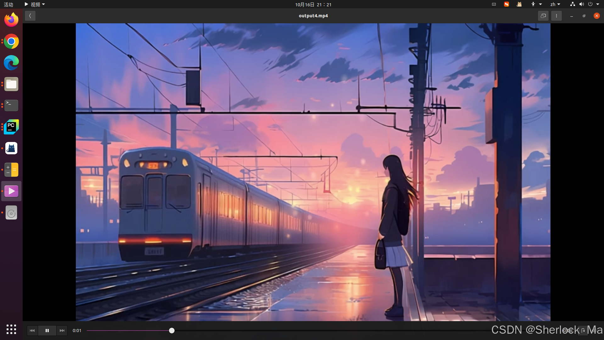
在I2V模式中，明显看到模型没有让裙子摆动，天色也没有暗下来，云彩也没用移动。火车和长发的移动效果令人满意。

此外，CogVideoX模型在视频的时长和分辨率方面还存在一些限制。虽然可以通过调整代码来尝试突破这些限制，但我们发现，一旦解除这些限制，生成的视频质量并不尽如人意。这表明模型在处理更高要求的视频内容时，仍需进一步的优化和提升，以满足用户对高质量视频生成的期待。我们期待随着技术的不断进步，未来能够带来更加卓越的视频生成效果。

5.总结

CogVideoX是由智谱AI推出的一款先进的视频生成模型，它通过深度学习和计算机视觉技术，能够将简短的文本描述或静态图片转化为高质量、具有视觉吸引力的动态视频。这一技术的出现极大地拓展了视频创作的边界，为用户提供了一种全新的视频创作体验。

CogVideoX的应用前景非常广阔，它不仅降低了技术门槛，使得更多的创作者和企业能够利用AI技术生成专业级别的视频内容，还在广告制作、影视后期、教育和研究等多个领域提供了强大的支持。例如，创作者可以利用CogVideoX生成独特的视频内容，企业可以提高视频生产效率，降低成本，教育机构和研究人员也可以探索视频生成技术的新领域。

此外，CogVideoX模型已经在智谱清言的PC端、移动应用端以及小程序端正式上线，所有C端用户均可通过智谱清言的AI视频生成功能“清影”体验AI文本生成视频和图像生成视频的服务。清影的主要特点包括快速生成、高效的指令遵循能力、内容连贯性和画面调度灵活性，能够满足用户在视频内容创作上的多样化需求。

总的来说，CogVideoX模型的开源无疑将推动AI视频生成技术的发展，开启视频创作的新纪元。无论是个人用户还是企业应用，CogVideoX都能提供丰富且富有创意的视频生成体验。
 

探索AI视频生成的无限可能，与CogVideoX一起开启创意之旅！如果你对这篇分享充满热情，别忘了点赞和关注，让我们的创新故事持续发光发热。每一次互动都是我们前进的动力，感谢你的支持，让我们共同见证科技与艺术的完美融合！