scGen perturbation response prediction

如何利用scGen进行扰动响应预测

scGen是什么

scGen is a generative model to predict single-cell perturbation response across cell types, studies and species (Nature Methods, 2019). scGen is implemented using the scvi-tools framework.

文章传送门

Original tutorial link

相比于原教程，本文主要是对部分步骤的意义进行了注解，方便对流程的理解。

流程

①导包

import logging
import scanpy as sc
import scgen

②准备数据集

train = sc.read("./tests/data/train_kang.h5ad",
                backup_url='https://drive.google.com/uc?id=1r87vhoLLq6PXAYdmyyd89zG90eJOFYLk')

train_new = train[~((train.obs["cell_type"] == "CD4T") &
                    (train.obs["condition"] == "stimulated"))]

数据类型还是Anndata数据。这里的数据是经过QC、normalize和log计算的，并且筛选出了HVG。在QC时，最好也排除掉TCR的相关基因，以保证模型的泛化性。

我们需要制作一个训练数据集和一个测试数据集，并且需要给数据标注上condition和cell_type。

其中condition只能有两种标签，分别代表响应状态和未响应状态，如’control’和’stimulated’。

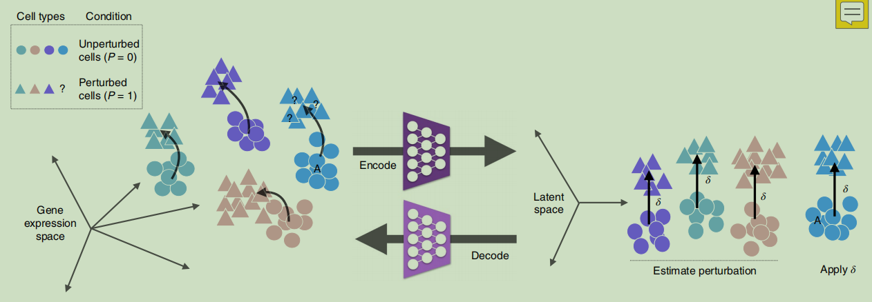
scGen就是用在latent space中学到的从control到stimulated的映射向量来进行perturbation response prediction的。

映射结果是RNA expression matrix。

如原理下图：

③模型训练

scgen.SCGEN.setup_anndata(train_new, batch_key="condition", labels_key="cell_type")

model = scgen.SCGEN(train_new)
model.train(
    max_epochs=100,
    batch_size=32,
    early_stopping=True,
    early_stopping_patience=25
)

# Save the trained model
model.save("../saved_models/model_perturbation_prediction.pt", overwrite=True)

查看latent space的数据分布

latent_X = model.get_latent_representation()
latent_adata = sc.AnnData(X=latent_X, obs=train_new.obs.copy())

sc.pp.neighbors(latent_adata)
sc.tl.umap(latent_adata)
sc.pl.umap(latent_adata, color=['condition', 'cell_type'], wspace=0.4, frameon=False)

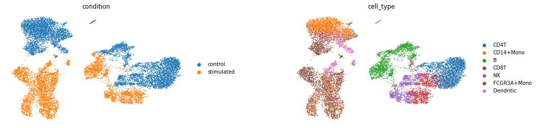
理想的情况应该是模型在隐层空间中对condition做出了较好的区分，这样模型才能有效的学到从control到stimulated的映射向量δ。

那么这个δ向量是怎么得到的呢。文章的做法其实非常简单。

对于每个细胞类型，我们对细胞类型大小进行上采样，以等于该条件下的最大细胞类型大小。对具有较高样本量的条件（control or stimulate）进行了随机降采样，以匹配其他条件的样本量。
将隐层向量分为两群，control和stimulate。分别求出control和stimulate的均值向量，用这两个均值向量作差，即可得出δ向量。

④预测

pred, delta = model.predict(
    ctrl_key='control',
    stim_key='stimulated',
    celltype_to_predict='CD4T'
)
pred.obs['condition'] = 'pred'

这里pred是预测得到的adata对象，delta是计算得出的δ映射向量。

⑤验证预测结果

PCA

ctrl_adata = train[((train.obs['cell_type'] == 'CD4T') & (train.obs['condition'] == 'control'))]
stim_adata = train[((train.obs['cell_type'] == 'CD4T') & (train.obs['condition'] == 'stimulated'))]

eval_adata = ctrl_adata.concatenate(stim_adata, pred)

sc.tl.pca(eval_adata)
sc.pl.pca(eval_adata, color="condition", frameon=False)

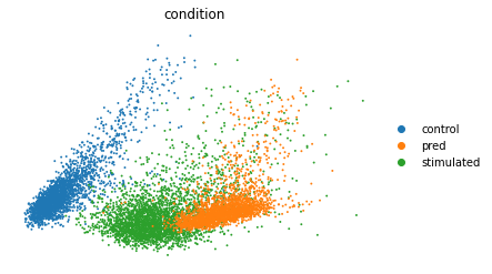
这里是通过绘制RNA表达矩阵PCA降维后的散点图来进行验证，由于我们的预测结果是stimulated，理想的情况下预测结果应该是靠近stimulated并远离control。

Mean correlation plot

Plots mean matching figure for a set of specific genes.

CD4T = train[train.obs["cell_type"] =="CD4T"]
sc.tl.rank_genes_groups(CD4T, groupby="condition", method="wilcoxon")
diff_genes = CD4T.uns["rank_genes_groups"]["names"]["stimulated"]
print(diff_genes)

r2_value = model.reg_mean_plot(
    eval_adata,
    axis_keys={"x": "pred", "y": "stimulated"},
    # list of gene names to be plotted.
    gene_list=diff_genes[:10],
    labels={"x": "predicted", "y": "ground truth"},
    path_to_save="./reg_mean1.pdf",
    show=True,
    legend=False
)

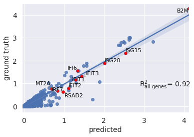
这里是用训练数据中的基因平均表达量作y，预测数据的基因平均表达量作x，作线性回归并计算决定系数$R^2$，$R^2$值越靠近1表示基因表达越相近。（这里是计算了全部基因的决定系数）

r2_value = model.reg_mean_plot(
    eval_adata,
    axis_keys={"x": "pred", "y": "stimulated"},
    gene_list=diff_genes[:10],
    top_100_genes= diff_genes,
    labels={"x": "predicted","y": "ground truth"},
    path_to_save="./reg_mean1.pdf",
    show=True,
    legend=False
)

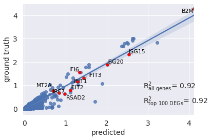
和上图不同，这里还额外计算了condition差异表达基因的决定系数。

个人的额外看法。
如果在上一步PCA的umap图中，预测结果距离control和stimulated的距离都差不多，那么在这一步也应该额外计算预测结果和control的决定系数，当出现和control做回归时的$R^2$值大于和stimulated的$R^2$值时，表示模型的训练失败，此时模型无法正确的预测出激活后的RNA表达矩阵。

Violin plot for a specific gene

sc.pl.violin(eval_adata, keys="ISG15", groupby="condition")

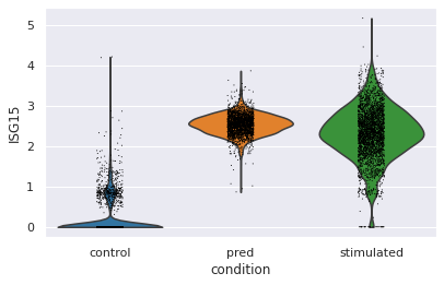
这里绘制了重点关注基因ISG15的琴谱图，可以看出预测结果的细胞分布和stimulated相似。

总结

scGen模型整体其实就分为两部分，VAE + 向量算法，VAE是采用的经典VAE模型，向量算法的计算是简单的用平均向量作差，两部分拆开来看都没有什么新奇和复杂的，但是模型的总体效果非常好。

在我自己实际使用时，预测效果并不太好，预测结果距离control比距离stimulated更近，这可能是由于训练数据的condition不是只受一种因素影响造成的。所以建议大家保证数据集的扰动因素有且只有一种。