梯度提升决策树GBDT及其sklearn实践

梯度提升综述

梯度提升树的同义叫法：

• GBDT，Gradient Boosting Decision Tree，梯度提升决策树
• GBRT，Gradient Boosting Regression Tree，梯度回归树
• MART，Multiple Additive Regression Tree，多重累加回归树

GBDT是一种迭代的决策树算法，由多棵回归决策树组成，将所有决策树的输出累加作为最终输出.即
$$f_m(\mathbf{x})=f_{m-1}(\mathbf{x})+T(\mathbf{x};{\Theta }_m)$$
对于回归问题，若采用平方误差损失，则
$$L(y,f_{m-1}({\mathbf{x}}_i)+T({\mathbf{x}}_i;{\Theta }_m))=[y-f_{m-1}(\mathbf{x})-T(\mathbf{x};{\Theta }_m){]}^2=[r-T(\mathbf{x};{\Theta }_m){]}^2$$

其中$r=y-f_{m-1}(\mathbf{x})$是当前模型在训练集上的残差（实际值-预测值），每轮基模型的学习实际是在拟合当前模型的残差。

GBDT算法使用 负梯度近似残差，基模型的学习问题转变为拟合当前总体损失负梯度，使得各损失函数可用。Sklearn的GBDT实现，回归问题可选用MSE、MAE、Huber等损失，分类问题可选用Deviance（二分类对应于logistic、多分类对应于softmax）、Exponential损失。

GBDT优缺点：

• 采用决策树作为基模型，不需要特征标准化，数值缩放不影响分裂点，而且树形模型不通过梯度下降求解；
• 模型解释力强；
• 适用于不同的损失函数；
• 计算密集型，不能并行计算；
• 无法处理高纬稀疏特征的数据，如词袋特征的文本数据；

GBDT for Regression and Binary Classification

算法实现步骤：

• 初始化，将使损失函数极小的常数值作为初始值（MSE损失初值为均值）：
  $$H_0(\mathbf{x})=\arg \underset{c}{\min }{\mathbb{E}}_{\mathcal{D}}[L(y,c)]=\arg \underset{c}{\min }\sum _i{w}_{i}L(y_i,c)$$

• $t$，从1至T遍历：

  • 将当前总体损失函数的负梯度作为本轮基模型拟合值：
    $$g_t=-{\left[\frac{\partial L(y,H(\mathbf{x}))}{\partial H(\mathbf{x})}\right]}_{H(\mathbf{x})=H_{t-1}(\mathbf{x})}$$

    回归任务一般使用MSE损失，分类任务一般使用Deviance损失（二分类和多分类对应于logistic和softmax）.

  • 使用CART决策树拟合$g_t$，分类/回归任务均可使用MSE损失，对应结点输出均值：
    $$h_t(\mathbf{x})=\arg \underset{h}{\min }{\mathbb{E}}_{\mathcal{D}}[(g_t-h(\mathbf{x}){)}^2]=\sum _{j=1}^J{\overline{y}}_j\mathbb{I}(\mathbf{x}\in R_j)$$

  • 搜索最优步长${\alpha }_t$（sklearn使用固定值learning_rate），组合基模型
    $$H_t(\mathbf{x})=H_{t-1}(\mathbf{x})+{\alpha }_t{h}_t(\mathbf{x}),{\alpha }_t=\arg \underset{\alpha }{\min }{\mathbb{E}}_{\mathcal{D}}[L(y,H_{t-1}(\mathbf{x})+\alpha h_t(\mathbf{x}))],$$

• 迭代结束，最终模型为：
  $$H(\mathbf{x})=H_0(\mathbf{x})+\sum _{t=1}^T{\alpha }_t{h}_t(\mathbf{x})$$

GBDT for K-class Classification

算法实现步骤：

• 初始化，各目标函数值初值为0，$f_{k0}(\mathbf{x})=0$；

• $t$，从1至T遍历：

  • $k$，从1至K遍历：

    • 将当前类别总体损失的负梯度作为本轮拟合值，若使用Deviance损失，则：
      $$g_{tk}=y_k-\frac{\exp (f_{t-1,k}(\mathbf{x}))}{{\sum }_{l=1}^K\exp (f_{t-1,l}(\mathbf{x}))}$$

    • 拟合CART回归树：
      $$h_{tk}(\mathbf{x})=\arg \underset{h}{\min }{\mathbb{E}}_{\mathcal{D}}[(g_{tk}-h_{tk}(\mathbf{x}){)}^2]$$

    • 根据最优步长${\alpha }_{tk}$组合基模型：
      $$f_{tk}(\mathbf{x})=f_{t-1,k}(\mathbf{x})+{\alpha }_{tk}{h}_{tk}(\mathbf{x})$$

• 迭代结束得K个模型，第k个模型：
  $$f_k(\mathbf{x})=\sum _{t=1}^T{\alpha }_{tk}{h}_{tk}(\mathbf{x})$$

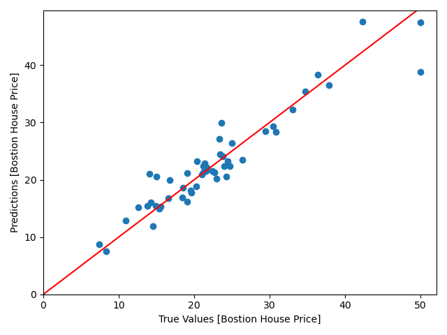
实例1：GBDT预测波士顿房价

from sklearn.ensemble import GradientBoostingRegressor
from sklearn.datasets import load_boston
from sklearn.model_selection import train_test_split
import matplotlib.pyplot as plt

dataset = load_boston()
features = dataset.feature_names

X_train, X_test, y_train, y_test = train_test_split(
    dataset.data, dataset.target, train_size=0.9, test_size=0.1, random_state=188)

gbr = GradientBoostingRegressor(
    loss='ls',
    learning_rate=0.1,
    n_estimators=500,
    max_depth=4,
    min_samples_split=2,
    verbose=1)

gbr.fit(X_train, y_train)

plt.scatter(y_test, gbr.predict(X_test))
plt.xlabel('True Values [Bostion House Price]')
plt.ylabel('Predictions [Bostion House Price]')
# plt.axis('equal')
# plt.axis('square')
plt.xlim([0, plt.xlim()[1]])
plt.ylim([0, plt.ylim()[1]])
plt.plot([-100, 100], [-100, 100], 'r')
plt.show()

模型预测效果图如下，离直线越近的点，拟合越好：

实例2：GBDT预测鸢尾花类别

import matplotlib.pyplot as plt
import seaborn as sns
from sklearn.datasets import load_iris
from sklearn.ensemble import GradientBoostingClassifier
from sklearn.metrics import classification_report, confusion_matrix
from sklearn.model_selection import train_test_split

dataset = load_iris()
features = dataset.feature_names

X_train, X_test, y_train, y_test = train_test_split(
    dataset.data, dataset.target, train_size=0.8, test_size=0.2, random_state=188)

gbc = GradientBoostingClassifier(
    loss='deviance',
    learning_rate=0.1,
    n_estimators=200,
    max_depth=4,
    min_samples_split=2,
    verbose=1)
gbc.fit(X_train, y_train)

y_pred = gbc.predict(X_test)
report = classification_report(y_test, gbc.predict(X_test), output_dict=False)
print(report)

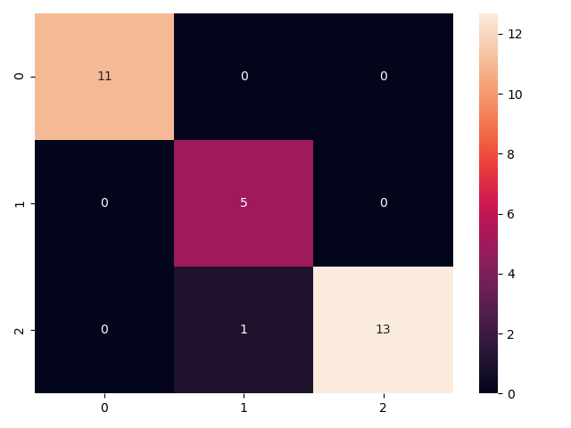
sns.heatmap(confusion_matrix(y_test, y_pred), annot=True, robust=True)
plt.show()

预测分类报告

              precision    recall  f1-score   support
           0       1.00      1.00      1.00        11
           1       0.83      1.00      0.91         5
           2       1.00      0.93      0.96        14
    accuracy                           0.97        30
   macro avg       0.94      0.98      0.96        30
weighted avg       0.97      0.97      0.97        30

预测分类混淆矩阵