DataWhale-(scikit-learn教程)-Task01(线性回归与逻辑回归)-202112

DataWhale-(scikit-learn教程)-Task01(线性回归与逻辑回归)-202112

DataWhale的scikit-learn教程链接
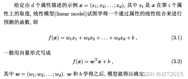
一、 线性回归
​​1. 线性回归的基本形式

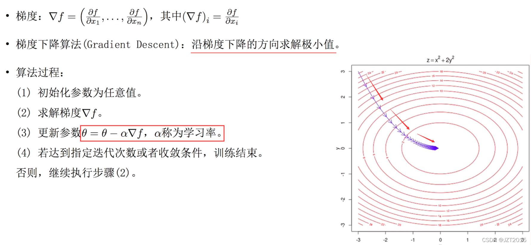
2. 梯度下降法训练

假设给定模型$h(\theta )={\sum }_{j=0}^n{\theta }_j{x}_j$以及目标函数(损失函数):$J(\theta )=\frac{1}{m}{\sum }_{i=0}^m{\left(h_{\theta }\left(x^i\right)-y^i\right)}^2$, 其中$m$表示数据的量，我们目标是为了$J(\theta )$尽可能小，所以这里加上$\frac{1}{2}$为了后面的简化，即$J(\theta )=\frac{1}{2m}{\sum }_{i=0}^m{\left(y^i-h_{\theta }\left(x^i\right)\right)}^2$。
那么梯度则为：
$$\begin{array}{rl}\frac{\partial J(\theta )}{\partial {\theta }_j}& =\frac{1}{m}\sum _{i=0}^m\left(y^i-h_{\theta }\left(x^i\right)\right)\frac{\partial }{\partial {\theta }_j}\left(y^i-h_{\theta }\left(x^i\right)\right)\\ & =-\frac{1}{m}\sum _{i=0}^m\left(y^i-h_{\theta }\left(x^i\right)\right)\frac{\partial }{\partial {\theta }_j}\left(\sum _{j=0}^n{\theta }_j{x}_j^i-y^i\right)\\ & =-\frac{1}{m}\sum _{i=0}^m\left(y^i-h_{\theta }\left(x^i\right)\right)x_j^i\\ & =\frac{1}{m}\sum _{i=0}^m\left(h_{\theta }(x^i)-y^i)\right)x_j^i\end{array}$$

设$x$是(m,n)维的矩阵，$y$是(m,1)维度的矩阵，$h_{\theta }$是预测的值，维度与$y$相同，那么梯度用矩阵表示如下:
$$\frac{\partial J(\theta )}{\partial {\theta }_j}=\frac{1}{m}{x}^T(h_{\theta }-y)$$

3. 一元线性回归代码实现
(1) numpy使用梯度下降实现

import numpy as np
import matplotlib.pyplot as plt

def true_fun(X):
    return 1.5*X + 0.2

np.random.seed(0) # 随机种子
n_samples = 30
'''生成随机数据作为训练集'''
X_train = np.sort(np.random.rand(n_samples)) 
y_train = (true_fun(X_train) + np.random.randn(n_samples) * 0.05).reshape(n_samples,1)
data_X = []
for x in X_train:
    data_X.append([1,x])
data_X = np.array((data_X))

m,p = np.shape(data_X) # m, 数据量 p: 特征数
max_iter = 1000 # 迭代数
weights = np.ones((p,1))  
alpha = 0.1 # 学习率
for i in range(0,max_iter):
    error = np.dot(data_X,weights)- y_train
    gradient = data_X.transpose().dot(error)/m
    weights = weights - alpha * gradient
print("输出参数w:",weights[1:][0]) # 输出模型参数w
print("输出参数:b",weights[0]) # 输出参数b

X_test = np.linspace(0, 1, 100)
plt.plot(X_test, X_test*weights[1][0]+weights[0][0], label="Model") 
plt.plot(X_test, true_fun(X_test), label="True function")
plt.scatter(X_train,y_train) # 画出训练集的点
plt.legend(loc="best")
plt.show()

(2) sklearn实现一元线性回归

import numpy as np
from sklearn.linear_model import LinearRegression # 导入线性回归模型
import matplotlib.pyplot as plt

def true_fun(X):
    return 1.5*X + 0.2

np.random.seed(0) # 随机种子
n_samples = 30
'''生成随机数据作为训练集'''
X_train = np.sort(np.random.rand(n_samples)) 
y_train = (true_fun(X_train) + np.random.randn(n_samples) * 0.05).reshape(n_samples,1)

model = LinearRegression() # 定义模型
model.fit(X_train[:,np.newaxis], y_train) # 训练模型

print("输出参数w:",model.coef_) # 输出模型参数w
print("输出参数:b",model.intercept_) # 输出参数b

X_test = np.linspace(0, 1, 100)
plt.plot(X_test, model.predict(X_test[:, np.newaxis]), label="Model")
plt.plot(X_test, true_fun(X_test), label="True function")
plt.scatter(X_train,y_train) # 画出训练集的点
plt.legend(loc="best")
plt.show()

(3) sklearn实现多元线性回归

from sklearn.linear_model import LinearRegression

X_train = [[1,1,1],[1,1,2],[1,2,1]]
y_train = [[6],[9],[8]]
 
model = LinearRegression()
model.fit(X_train, y_train)
print("输出参数w:",model.coef_) # 输出参数w1,w2,w3
print("输出参数b:",model.intercept_) # 输出参数b
test_X = [[1,3,5]]
pred_y = model.predict(test_X)
print("预测结果:",pred_y)

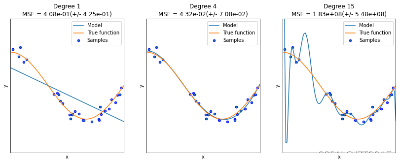
二、多项式回归以及过拟合与欠拟合

1. 训练集
   用来训练模型内参数的数据集
2. 验证集
   用于在训练过程中检验模型的状态，收敛情况，通常用于调整超参数，根据几组模型验证集上的表现决定哪组超参数拥有最好的性能。同时验证集在训练过程中还可以用来监控模型是否发生过拟合，一般来说验证集表现稳定后，若继续训练，训练集表现还会继续上升，但是验证集会出现不升反降的情况，这样一般就发生了过拟合。所以验证集也用来判断何时停止训练。
3. 测试集
   测试集用来评价模型泛化能力，即使用训练集调整了参数，之前模型使用验证集确定了超参数，最后使用一个不同的数据集来检查模型。
4. 交叉验证
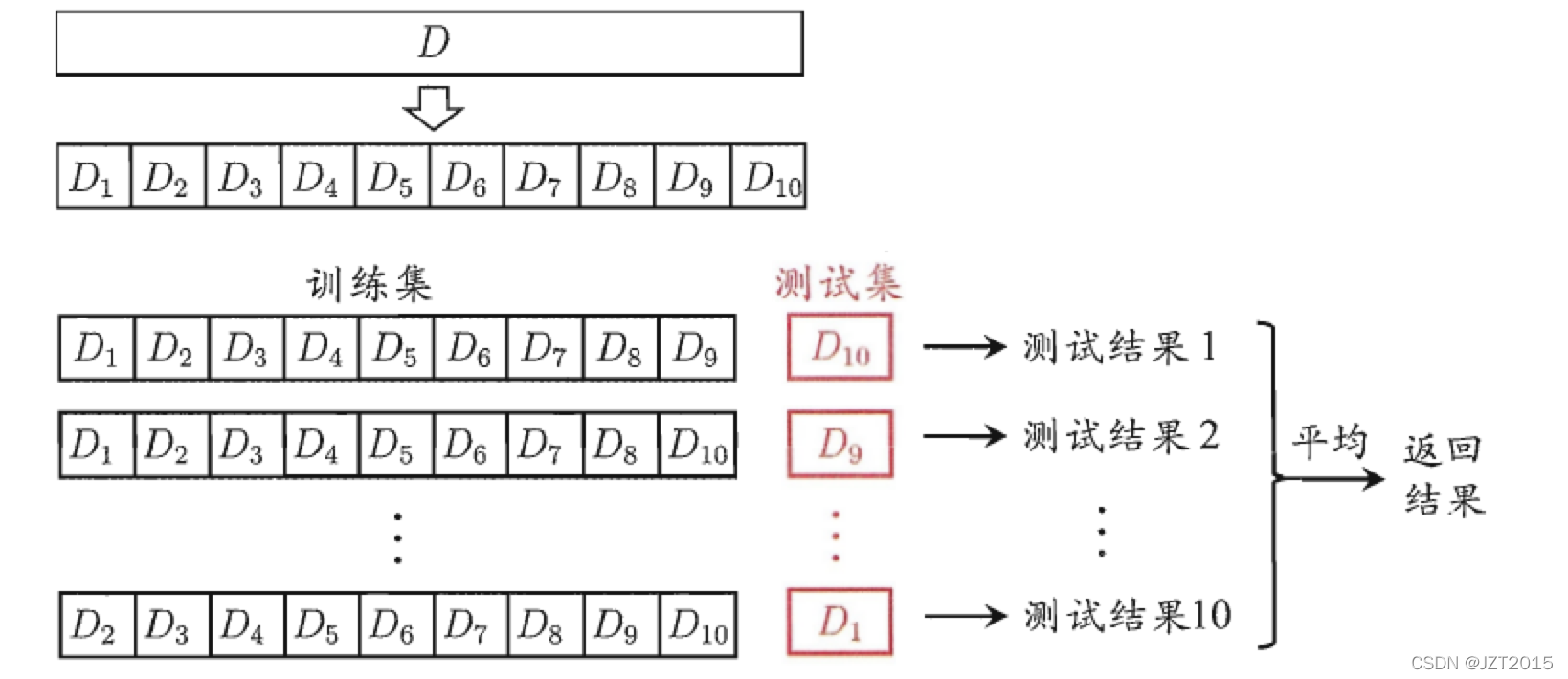
   交叉验证法的作用就是尝试利用不同的训练集/测试集划分来对模型做多组不同的训练/测试，来应对测试结果过于片面以及训练数据不足的问题。
   
5. 多项式回归的sklearn实现

import numpy as np
import matplotlib.pyplot as plt
from sklearn.pipeline import Pipeline
from sklearn.preprocessing import PolynomialFeatures
from sklearn.linear_model import LinearRegression
from sklearn.model_selection import cross_val_score

def true_fun(X):
    return np.cos(1.5 * np.pi * X)
np.random.seed(0)

n_samples = 30
degrees = [1, 4, 15] # 多项式最高次

X = np.sort(np.random.rand(n_samples)) 
y = true_fun(X) + np.random.randn(n_samples) * 0.1

plt.figure(figsize=(14, 5))
for i in range(len(degrees)):
    ax = plt.subplot(1, len(degrees), i + 1)
    plt.setp(ax, xticks=(), yticks=())

    polynomial_features = PolynomialFeatures(degree=degrees[i],
                                             include_bias=False)
    linear_regression = LinearRegression()
    pipeline = Pipeline([("polynomial_features", polynomial_features),
                         ("linear_regression", linear_regression)]) # 使用pipline串联模型
    pipeline.fit(X[:, np.newaxis], y)

    # 使用交叉验证
    scores = cross_val_score(pipeline, X[:, np.newaxis], y,
                             scoring="neg_mean_squared_error", cv=10)
    X_test = np.linspace(0, 1, 100)
    plt.plot(X_test, pipeline.predict(X_test[:, np.newaxis]), label="Model")
    plt.plot(X_test, true_fun(X_test), label="True function")
    plt.scatter(X, y, edgecolor='b', s=20, label="Samples")
    plt.xlabel("x")
    plt.ylabel("y")
    plt.xlim((0, 1))
    plt.ylim((-2, 2))
    plt.legend(loc="best")
    plt.title("Degree {}\nMSE = {:.2e}(+/- {:.2e})".format(
        degrees[i], -scores.mean(), scores.std()))
plt.show()

二、逻辑回归

同线性回归一样，需要求出$n$个参数：

$$z={\theta }_0+{\theta }_{1}x+{\theta }_{2}x+...+{\theta }_{n}x={\theta }^{T}x$$

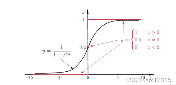
逻辑回归通过Sigmoid函数引入了非线性因素，可以轻松处理二分类问题:

$$h_{\theta }(x)=g\left({\theta }^{T}x\right),g(z)=\frac{1}{1+e^{-z}}$$

与线性回归不同，逻辑回归使用的是交叉熵损失函数:

$$J(\theta )=-\frac{1}{m}[\sum _{i=1}^m\left(y^{(i)}\log h_{\theta }\left(x^{(i)}\right)+\left(1-y^{(i)}\right)\log \left(1-h_{\theta }\left(x^{(i)}\right)\right)\right]$$

其梯度为:

$$\frac{\partial J(\theta )}{\partial {\theta }_j}=\frac{1}{m}\sum _{i=0}^m\left(h_{\theta }-y^i\left(x^i\right)\right)x_j^i$$

形式和线性回归一样，但其实假设函数(Hypothesis function)不一样，逻辑回归是:
$$h_{\theta }(x)=\frac{1}{1+e^{-{\theta }^{T}x}}$$

其推导如下:

$$\begin{array}{rl}\frac{\partial }{\partial {\theta }_j}J(\theta )& =\frac{\partial }{\partial {\theta }_j}\left[-\frac{1}{m}\sum _{i=1}^m\left[y^{(i)}\log \left(h_{\theta }\left(x^{(i)}\right)\right)+\left(1-y^{(i)}\right)\log \left(1-h_{\theta }\left(x^{(i)}\right)\right)\right]\right]\\ & =-\frac{1}{m}\sum _{i=1}^m\left[y^{(i)}\frac{1}{h_{\theta }\left(x^{(i)}\right))}\frac{\partial }{\partial {\theta }_j}{h}_{\theta }\left(x^{(i)}\right)-\left(1-y^{(i)}\right)\frac{1}{1-h_{\theta }\left(x^{(i)}\right)}\frac{\partial }{\partial {\theta }_j}{h}_{\theta }\left(x^{(i)}\right)\right]\\ & =-\frac{1}{m}\sum _{i=1}^m\left[y^{(i)}\frac{1}{h_{\theta }\left(x^{(i)}\right))}-\left(1-y^{(i)}\right)\frac{1}{1-h_{\theta }\left(x^{(i)}\right)}\right]\frac{\partial }{\partial {\theta }_j}{h}_{\theta }\left(x^{(i)}\right)\\ & =-\frac{1}{m}\sum _{i=1}^m\left[y^{(i)}\frac{1}{h_{\theta }\left(x^{(i)}\right))}-\left(1-y^{(i)}\right)\frac{1}{1-h_{\theta }\left(x^{(i)}\right)}\right]\frac{\partial }{\partial {\theta }_j}g\left({\theta }^T{x}^{(i)}\right)\end{array}$$

因为:
$$\begin{array}{rl}\frac{\partial }{\partial {\theta }_j}g\left({\theta }^T{x}^{(i)}\right)& =\frac{\partial }{\partial {\theta }_j}\frac{1}{1+e^{-{\theta }^T{x}^{(i)}}}\\ & =\frac{e^{-{\theta }^T{x}^{(i)}}}{{\left(1{+}^{-\theta }{T}^{T_x(i)}\right)}^2}\frac{\partial }{\partial {\theta }_j}{\theta }^T{x}^{(i)}\\ & =g\left({\theta }^T{x}^{(i)}\right)\left(1-g\left({\theta }^T{x}^{(i)}\right)\right)x_j^{(i)}\end{array}$$
所以:
$$\begin{array}{rl}\frac{\partial }{\partial {\theta }_j}J(\theta )& =-\frac{1}{m}\sum _{i=1}^m\left[y^{(i)}\left(1-g\left({\theta }^T{x}^{(i)}\right)\right)-\left(1-y^{(i)}\right)g\left({\theta }^T{x}^{(i)}\right)\right]x_j^{(i)}\\ & =-\frac{1}{m}\sum _{i=1}^m\left(y^{(i)}-g\left({\theta }^T{x}^{(i)}\right)\right)x_j^{(i)}\\ & =\frac{1}{m}\sum _{i=1}^m\left(h_{\theta }\left(x^{(i)}\right)-y^{(i)}\right)x_j^{(i)}\end{array}$$

1. 逻辑回归用numpy实现

import sys,os
curr_path = os.path.dirname(os.path.abspath(__file__)) # 当前文件所在绝对路径
parent_path = os.path.dirname(curr_path) # 父路径
sys.path.append(parent_path) # 添加路径到系统路径

from Mnist.load_data import load_local_mnist

import numpy as np
import time


class LogisticRegression:
    def __init__(self, x_train, y_train, x_test, y_test):
        '''
        Args:
            x_train [Array]: 训练集数据
            y_train [Array]: 训练集标签
            x_test [Array]: 测试集数据
            y_test [Array]: 测试集标签
        '''
        self.x_train, self.y_train = x_train, y_train
        self.x_test, self.y_test = x_test, y_test
        # 将输入数据转为矩阵形式，方便运算
        self.x_train_mat, self.x_test_mat = np.mat(
            self.x_train), np.mat(self.x_test)
        self.y_train_mat, self.y_test_mat = np.mat(
            self.y_test).T, np.mat(self.y_test).T
        # theta表示模型的参数，即w和b
        self.theta = np.mat(np.zeros(len(x_train[0])))
        self.lr=0.001 # 可以设置学习率优化，使用Adam等optimizier
        self.n_iters=10  # 设置迭代次数
    @staticmethod
    def sigmoid(x):
        '''sigmoid函数
        '''
        return 1.0/(1+np.exp(-x))
        
    def _predict(self,x_test_mat):
        P=self.sigmoid(np.dot(x_test_mat, self.theta.T))
        if P >= 0.5:
            return 1
        return 0
    def train(self):
        '''训练过程，可参考伪代码
        '''
        for i_iter in range(self.n_iters):
            for i in range(len(self.x_train)):
                result = self.sigmoid(np.dot(self.x_train_mat[i], self.theta.T))
                error = self.y_train[i]- result
                grad = error*self.x_train_mat[i]
                self.theta+= self.lr*grad
            print('LogisticRegression Model(learning_rate={},i_iter={})'.format(
            self.lr, i_iter+1))
    def save(self):
        '''保存模型参数到本地文件
        '''
        np.save(os.path.dirname(sys.argv[0])+"/theta.npy",self.theta)
    def load(self):
        self.theta=np.load(os.path.dirname(sys.argv[0])+"/theta.npy")
    def test(self):
         # 错误值计数
        error_count = 0
        #对于测试集中每一个测试样本进行验证
        for n in range(len(self.x_test)):
            y_predict=self._predict(self.x_test_mat[n])
            #如果标记与预测不一致，错误值加1
            if self.y_test[n] != y_predict:
                error_count += 1
            print("accuracy=",1 - (error_count /(n+1)))
        #返回准确率
        return 1 - error_count / len(self.x_test)

def normalized_dataset():
    # 加载数据集，one_hot=False意思是输出标签为数字形式，比如3而不是[0,0,0,1,0,0,0,0,0,0]
    (x_train, y_train), (x_test, y_test) = load_local_mnist(one_hot=False)
    # 将w和b结合在一起，因此训练数据增加一维
    ones_col=[[1] for i in range(len(x_train))] # 生成全为1的二维嵌套列表，即[[1],[1],...,[1]]
    x_train_modified=np.append(x_train,ones_col,axis=1)
    ones_col=[[1] for i in range(len(x_test))] # 生成全为1的二维嵌套列表，即[[1],[1],...,[1]]
    x_test_modified=np.append(x_test,ones_col,axis=1)
    # Mnsit有0-9是个标记，由于是二分类任务，所以将标记0的作为1，其余为0
    # 验证过<5为1 >5为0时正确率在90%左右，猜测是因为数多了以后，可能不同数的特征较乱，不能有效地计算出一个合理的超平面
    # 查看了一下之前感知机的结果，以5为分界时正确率81，重新修改为0和其余数时正确率98.91%
    # 看来如果样本标签比较杂的话，对于是否能有效地划分超平面确实存在很大影响
    y_train_modified=np.array([1 if y_train[i]==1 else 0 for i in range(len(y_train))])
    y_test_modified=np.array([1 if y_test[i]==1 else 0 for i in range(len(y_test))])
    return x_train_modified,y_train_modified,x_test_modified,y_test_modified

if __name__ == "__main__":
    start = time.time()   
    x_train_modified,y_train_modified,x_test_modified,y_test_modified = normalized_dataset()
    model=LogisticRegression(x_train_modified,y_train_modified,x_test_modified,y_test_modified)
    model.train()
    model.save()
    model.load()
    accur=model.test()
    end = time.time()
    print("total acc:",accur)
    print('time span:', end - start)

2. 逻辑回归用sklearn实现

import sys
from pathlib import Path
curr_path = str(Path().absolute())
parent_path = str(Path().absolute().parent)
sys.path.append(parent_path) # add current terminal path to sys.path

from Mnist.load_data import load_local_mnist

from sklearn.linear_model import LogisticRegression
from sklearn.metrics import classification_report

(X_train, y_train), (X_test, y_test) = load_local_mnist(normalize = False,one_hot = False)
model = LogisticRegression()
model.fit(X_train, y_train)
y_pred = model.predict(X_test)
print(classification_report(y_test, y_pred)) # 打印报告

import sys
from pathlib import Path
curr_path = str(Path().absolute())
parent_path = str(Path().absolute().parent)
sys.path.append(parent_path) # add current terminal path to sys.path

from Mnist.load_data import load_local_mnist

from sklearn.linear_model import LogisticRegression
from sklearn.metrics import classification_report

(X_train, y_train), (X_test, y_test) = load_local_mnist(normalize = False,one_hot = False)

X_train, y_train= X_train[:2000], y_train[:2000] 
X_test, y_test = X_test[:200],y_test[:200]

# solver：即使用的优化器，lbfgs：拟牛顿法， sag：随机梯度下降
model = LogisticRegression(solver='lbfgs', max_iter=500) # lbfgs：拟牛顿法
model.fit(X_train, y_train)
y_pred = model.predict(X_test)
print(classification_report(y_test, y_pred)) # 打印报告