Improving the way neural networks learn

LINK

Why sigmoid + quadratic cost function learning slow?

The quadratic cost function is given by

$$C=\frac {(y-a)^2}{2} \tag 1$$
where $a$ is the neuron’s output. $a=\sigma (z)$, where $z=wx+b$. Using the chain rule to differentiate with respect to the weight and bias we get
$$\frac{\partial C}{\partial w} = (a-y)\sigma'(z) x = a \sigma'(z) \tag{2}$$
$$\frac{\partial C}{\partial b} = (a-y)\sigma'(z) = a \sigma'(z) \tag{3}$$
where I have substituted $x=1$ and $y=0$.
Recall the shape of the $\sigma$ function:

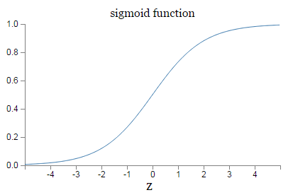
We can see from this graph that when the neuron’s output is close to 1, the curve gets very flat, and so $\sigma '(z)$ gets very small. Equations (2) and (3) then tell us that $\partial C/\partial w$ and $\partial C/\partial b$ get very small.

Using the quadratic cost when we have linear neurons in the output layer. Suppose that we have a many-layer multi-neuron network. Suppose all the neurons in the final layer are linear neurons, meaning that the sigmoid activation function is not applied, and the outputs are simply $a^L_j=z^L_j$. Show that if we use the quadratic cost function then the output error $δ^L$ for a single training example $x$ is given by

$$δ^L=a^L−y$$
Similarly to the previous problem, use this expression to show that the partial derivatives with respect to the weights and biases in the output layer are given by

$$\begin{eqnarray} \frac{\partial C}{\partial w^L_{jk}} & = & \frac{1}{n} \sum_x a^{L-1}_k (a^L_j-y_j) \\ \frac{\partial C}{\partial b^L_{j}} & = & \frac{1}{n} \sum_x (a^L_j-y_j). \end{eqnarray}$$
This shows that if the output neurons are linear neurons then the quadratic cost will not give rise to any problems with a learning slowdown. In this case the quadratic cost is, in fact, an appropriate cost function to use.

sigmoid + cross-entropy cost function

The cross-entropy cost function

$$C = -\frac{1}{n} \sum_x \left[y \ln a + (1-y ) \ln (1-a) \right] \tag 4$$
where $n$ is the total number of items of training data, the sum is over all training inputs, $x$, and $y$ is the corresponding desired output.

The partial derivative of the cross-entropy cost with respect to the weights. We substitute $a=\partial (z)$ into (4), and apply the chain rule twice, obtaining:

$$\begin{eqnarray} \frac{\partial C}{\partial w_j} & = & -\frac{1}{n} \sum_x \left( \frac{y }{\sigma(z)} -\frac{(1-y)}{1-\sigma(z)} \right) \frac{\partial \sigma}{\partial w_j} \tag{5}\\ & = & -\frac{1}{n} \sum_x \left( \frac{y}{\sigma(z)} -\frac{(1-y)}{1-\sigma(z)} \right)\sigma'(z) x_j. \tag{6}\end{eqnarray}$$
Putting everything over a common denominator and simplifying this becomes:
$$\begin{eqnarray} \frac{\partial C}{\partial w_j} & = & \frac{1}{n} \sum_x \frac{\sigma'(z) x_j}{\sigma(z) (1-\sigma(z))} (\sigma(z)-y). \tag{7}\end{eqnarray}$$
Using the definition of the sigmoid function, $\sigma(z) =1/(1+e^{-z})$, and a little algebra we can show that $\sigma'(z) =\sigma(z)(1-\sigma(z))$.
We see that the $\sigma ' (z)$ and $\sigma (z)(1-\sigma (z))$ terms cancel in the equation just above, and it simplifies to become:
$$\begin{eqnarray} \frac{\partial C}{\partial w_j} = \frac{1}{n} \sum_x x_j(\sigma(z)-y). \tag{8}\end{eqnarray}$$
This is a beautiful expression. It tells us that the rate at which the weight learns is controlled by $σ(z)−y$, i.e., by the error in the output. The larger the error, the faster the neuron will learn. In particular, it avoids the learning slowdown caused by the $σ′(z)$ term in the analogous equation for the quadratic cost, Equation (2).

In a similar way, we can compute the partial derivative for the bias.

$$\begin{eqnarray} \frac{\partial C}{\partial b} = \frac{1}{n} \sum_x (\sigma(z)-y). \tag{9}\end{eqnarray}$$

It’s easy to generalize the cross-entropy to many-neuron multi-layer networks. In particular, suppose $y=y_1,y_2,...$ are the desired values at the output neurons, i.e., the neurons in the final layer, while $a^L_1,a^L_2,...$ are the actual output values. Then we define the cross-entropy by

$$\begin{eqnarray} C = -\frac{1}{n} \sum_x \sum_j \left[y_j \ln a^L_j + (1-y_j) \ln (1-a^L_j) \right]. \end{eqnarray}$$

Softmax + log-likelihood cost

In a softmax layer we apply the so-called $softmax function$ to the $z^L_j$. According to this function, the activation $a^L_j$ of the $j$th output neuron is

$$\begin{eqnarray} a^L_j = \frac{e^{z^L_j}}{\sum_k e^{z^L_k}}, \tag{10}\end{eqnarray}$$
where in the denominator we sum over all the output neurons.

The log-likelihood cost:

$$\begin{eqnarray} C \equiv -\ln a^L_y. \tag{11}\end{eqnarray}$$

The partial derivative:

$$\begin{eqnarray} \frac{\partial C}{\partial b^L_j} & = & a^L_j-y_j \tag{12}\\ \frac{\partial C}{\partial w^L_{jk}} & = & a^{L-1}_k (a^L_j-y_j) \tag{13}\end{eqnarray}$$
These expressions ensure that we will not encounter a learning slowdown. In fact, it’s useful to think of a softmax output layer with log-likelihood cost as being quite similar to a sigmoid output layer with cross-entropy cost.

Given this similarity, should you use a sigmoid output layer and cross-entropy, or a softmax output layer and log-likelihood? In fact, in many situations both approaches work well. As a more general point of principle, softmax plus log-likelihood is worth using whenever you want to interpret the output activations as probabilities. That’s not always a concern, but can be useful with classification problems (like MNIST) involving disjoint classes.

overfitting

In general, one of the best ways of reducing overfitting is to increase the size of the training data. With enough training data it is difficult for even a very large network to overfit.