FlashAttention/ PagedAttention原理,大模型加速

1.1 GPU 硬件特点

由于 FlashAttention 计算 self-attention 的主要关键是有效的硬件使用，所以了解GPU内存和各种操作的性能特征是很有必要的。

以 A100 (40GB HBM) 为例，下面显示其内存层次结构的粗略图。SRAM内存分布在108个流式多处理器(SMs)上，每个处理器192KB。片上SRAM比HBM快得多，但比HBM小得多，在计算方面，使用Tensor Core的BFLOAT16 的理论峰值吞吐量为 312 TFLOPS。GPU 的典型操作方式是使用大量的线程来执行一个操作，这个操作被称为内核。输入从HBM加载到寄存器和SRAM，并在计算后写回HBM。

算法对于内存带宽的需求通常使用 计算强度 (arithmetic intensity) 来表示，单位是 OPs/byte。意思是在算法中平均每读入单位数据，能支持多少次运算操作。它有助于理解操作的瓶颈，即计算约束(Compute-bound)或带宽约束(Bandwidth-bound, or Memory-bound)。

• 算力 π ：也称为计算平台的性能上限，指的是一个计算平台倾尽全力每秒钟所能完成的浮点运算数。单位是 FLOPS or FLOP/s。
• 带宽 β ：也即计算平台的带宽上限，指的是一个计算平台倾尽全力每秒所能完成的内存交换量。单位是Byte/s。
• 计算强度上限 Imax=πβ ：两个指标相除即可得到计算平台的计算强度上限。它描述的是在这个计算平台上，单位内存交换最多用来进行多少次计算。单位是FLOPs/Byte。
• 模型的理论性能 P：我们最关心的指标，即模型_在计算平台上_所能达到的每秒浮点运算次数（理论值）。单位是FLOPSorFLOP/s。

如下图所示，Roof-line 描述了模型在一个计算平台的限制下，到底能达到多快的浮点计算速度，即算力决定“屋顶”的高度（绿色线段），带宽决定“房檐”的斜率（红色线段）。

Roof-line 划分出的两个瓶颈区域，即

• 计算约束——此时HBM访问所花费的时间相对较低，不管模型的计算强度 I 有多大，它的理论性能 P 最大只能等于计算平台的算力π。例如，具有较大内维数的矩阵乘法和具有大量通道的卷积。
• 带宽约束——当模型的计算强度 I 小于计算平台的计算强度上限 Imax 时，由于此时模型位于“房檐”区间，因此模型理论性能 P 的大小完全由计算平台的带宽上限 β（房檐的斜率）以及模型自身的计算强度 I 所决定。例如，elementwise 操作 (如activation, dropout 等) 和 规约操作 (如sum, softmax, batch normalization, layer normalization等)。

在 self-attention 中，计算速度比内存速度快得多，因此进程(操作)越来越多地受到内存(HBM)访问的瓶颈。因此，FlashAttention论文的目标是尽可能高效地使用SRAM来加快计算速度

1.2 FlashAttention 的核心思想及细节推导

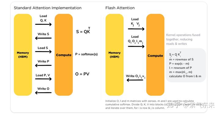
首先我们回顾一下标准 Attention 的操作:

其中 S,P （对于decoder来说还有 mask）的空间复杂度都是 O(N2) ，另外还有几个带宽约束的操作：对 S 的 scale, mask 和 softmax 操作，对 P 的 dropout 操作。下图算法展示了 HBM 与 SRAM 之间的数据传输过程。

1.2.1 FlashAttention 的优化思路

从上面的分析可以看出，O(N2)复杂度的矩阵对HBM及其重复读写是一个主要瓶颈。要解决这个问题，需要做两件主要的事情：

• 在不访问整个输入的情况下计算 softmax
• 不为反向传播存储大的中间 attention 矩阵

为此 FlashAttention 提出了两种方法来分布解决上述问题：tiling 和 recomputation。

• tiling - 注意力计算被重新构造，将输入分割成块，并通过在输入块上进行多次传递来递增地执行softmax操作。
• recomputation - 存储来自前向的 softmax 归一化因子，以便在反向中快速重新计算芯片上的 attention，这比从HBM读取中间矩阵的标准注意力方法更快。

由于重新计算，这确实导致FLOPs增加，但是由于大量减少HBM访问，FlashAttention运行速度更快(在GPT-2上高达7.6倍)。下面将详细推导 FlashAttention 的细节。

该算法背后的主要思想是分割输入，将它们从慢速HBM加载到快速SRAM，然后计算这些块的 attention 输出。在将每个块的输出相加之前，将其按正确的归一化因子进行缩放，从而得到正确的结果。

下面将分别讨论 tiling 和 recomputation 的正确性：

1.2.2 Tiling 与前向计算

上述算法中除了线性操作和 elementwise 外，分块计算注意力的关键部分是 softmax 的分块计算。向量的 softmax 可以计算为
$$\begin{gathered} m(x):=\underset{i}{\max }{x}_i \\ f(x):=\left[\begin{array}{lll}{e}^{x_1-m(x)}& \dots & e^{x_B-m(x)}\end{array}\right] \\ \ell (x):=\sum _{i}f(x{)}_i \\ \mathrm{softmax}(x):=\frac{f(x)}{\ell (x)} \end{gathered}$$

其中 x 可分解为 x=[x(1)x(2)]∈R2B ， x(1),x(2)∈RB 那么则有

$$m(x)=m\left(\left[x^{(1)}{x}^{(2)}\right]\right)=\max \left(m\left(x^{(1)}\right),m\left(x^{(2)}\right)\right)$$

那么可以通过如下构造的方式，使得 f(x) 的结果与分块前保持统一：

$$\begin{array}{rl}f(x)& =\left[\begin{array}{ll}{e}^{m\left(x^{(1)}\right)-m(x)}f\left(x^{(1)}\right)& e^{m\left(x^{(2)}\right)-m(x)}f\left(x^{(2)}\right)\end{array}\right]\\ & =\left[\begin{array}{ll}{e}^{m\left(x^{(1)}\right)-m(x)}\left[\begin{array}{lll}{e}^{x_1^{(1)}-m(x^{(1)})}& \dots & e^{x_B^{(1)}-m(x^{(1)})}\end{array}\right]& e^{m\left(x^{(2)}\right)-m(x)}\left[\begin{array}{lll}{e}^{x_1^{(2)}-m(x^{(2)})}& \dots & e^{x_B^{(2)}-m(x^{(2)})}\end{array}\right]\end{array}\right]\\ & =\left[\begin{array}{ll}\left[\begin{array}{lll}{e}^{x_1^{(1)}-m(x)}& \dots & e^{x_B^{(1)}-m(x)}\end{array}\right]& \left[\begin{array}{lll}{e}^{x_1^{(2)}-m(x)}& \dots & e^{x_B^{(2)}-m(x)}\end{array}\right]\end{array}\right]\\ & =\left[\begin{array}{lll}{e}^{x_1-m(x)}& \dots & e^{x_B-m(x)}\end{array}\right]\end{array}$$

ℓ(x) 的构造方式同理：

$$\ell (x)=\ell \left(\left[x^{(1)}{x}^{(2)}\right]\right)=e^{m\left(x^{(1)}\right)-m(x)}\ell \left(x^{(1)}\right)+e^{m\left(x^{(2)}\right)-m(x)}\ell \left(x^{(2)}\right)$$

由此 softmax⁡(x) 的结果自然与分块前保持统一：

$$\mathrm{softmax}(x)=\frac{f(x)}{\ell (x)}$$

softmax 的分块计算解决后，实际上其他部分的分块计算就简单多了，那么我们可以看下完整的 decoder 的 attention 的计算过程：

$$\begin{array}{rl}(1)& \mathbf{S}=\mathbf{Q}{\mathbf{K}}^{\top }/\sqrt{d}\in {\mathbb{R}}^{N\times N}\\ (2)& {\mathbf{S}}^{\text{masked }}=\mathrm{MASK}(\mathbf{S})\in {\mathbb{R}}^{N\times N}\\ (3)& \mathbf{P}=\mathrm{softmax}\left({\mathbf{S}}^{\text{masked }}\right)\in {\mathbb{R}}^{N\times N}\\ (4)& {\mathbf{P}}^{\text{dropped }}=\mathrm{dropout}\left(\mathbf{P},p_{\text{drop }}\right)\in {\mathbb{R}}^{N\times N}\\ (5)& \mathbf{O}={\mathbf{P}}^{\text{dropped }}\mathbf{V}\in {\mathbb{R}}^{N\times d}\end{array}$$

那么 FlashAttention 前向过程的算法可描述如下：

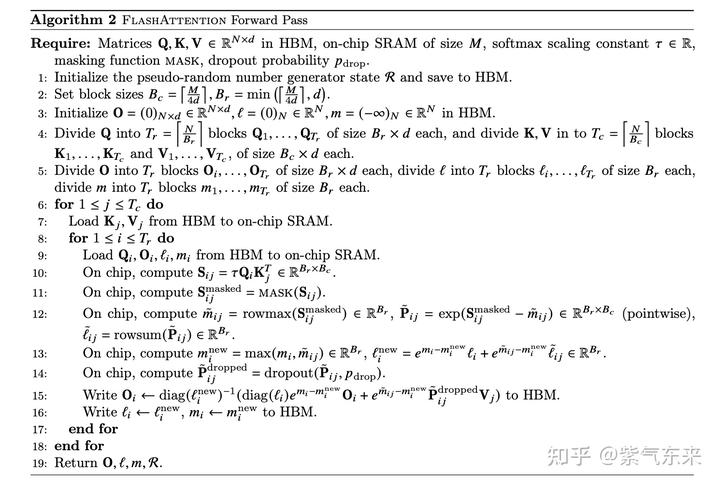
上述算法并没有增加额外计算（只是将大的操作拆成多个分块逐步计算），因此其算法复杂度仍为 O(N2d) ，另外由于增加了变量 ℓ,m ，因此空间复杂度增加 O(N) 。

其中第15行需要专门来推导一下，为简洁起见，先不考虑 mask 和 dropout 操作：

$\begin{array}{rl}{\mathbf{O}}_i^{(j+1)}& ={\mathbf{P}}_{i,:j+1}{\mathbf{V}}_{:j+1}=\mathrm{softmax}\left({\mathbf{S}}_{i,:j+1}\right){\mathbf{V}}_{:j+1}\\ & =\mathrm{diag}{\left({\ell }^{(j+1)}\right)}^{-1}\left(\exp \left(\left[\begin{array}{ll}{\mathbf{S}}_{i,:j}& {\mathbf{S}}_{i,j:j+1}\end{array}\right]-m^{(j+1)}\right)\right)\left[\begin{array}{c}{\mathbf{V}}_{:j}\\ {\mathbf{V}}_{j:j+1}\end{array}\right]\\ & =\mathrm{diag}{\left({\ell }^{(j+1)}\right)}^{-1}\left(\exp \left({\mathbf{S}}_{i,:j}-m^{(j+1)}\right){\mathbf{V}}_{:j}+\exp \left({\mathbf{S}}_{i,j:j+1}-m^{(j+1)}\right){\mathbf{V}}_{j:j+1}\right)\\ & =\mathrm{diag}{\left({\ell }^{(j+1)}\right)}^{-1}\left(e^{-m^{(j+1)}}\exp \left({\mathbf{S}}_{i,:j}\right){\mathbf{V}}_{:j}+e^{-m^{(j+1)}}\exp \left({\mathbf{S}}_{i,j:j+1}\right){\mathbf{V}}_{j:j+1}\right)\\ & =\mathrm{diag}{\left({\ell }^{(j+1)}\right)}^{-1}\left(\mathrm{diag}\left({\ell }^{(j)}\right)e^{m^{(j)}-m^{(j+1)}}\mathrm{diag}{\left({\ell }^{(j)}\right)}^{-1}\exp \left({\mathbf{S}}_{i,:j}-m^{(j)}\right){\mathbf{V}}_{:j}+e^{-m^{(j+1)}}\exp \left({\mathbf{S}}_{i,j:j+1}\right){\mathbf{V}}_{j:j+1}\right)\\ & =\mathrm{diag}{\left({\ell }^{(j+1)}\right)}^{-1}\left(\mathrm{diag}\left({\ell }^{(j)}\right)e^{m^{(j)}-m^{(j+1)}}{\mathbf{P}}_{i,:j}{\mathbf{V}}_{:j}+e^{-m^{(j+1)}}\exp \left({\mathbf{S}}_{i,j:j+1}\right){\mathbf{V}}_{j:j+1}\right)\\ & =\mathrm{diag}{\left({\ell }^{(j+1)}\right)}^{-1}\left(\mathrm{diag}\left({\ell }^{(j)}\right)e^{m^{(j)}-m^{(j+1)}}{\mathbf{O}}_i^{(j)}+e^{\tilde{m}-m^{(j+1)}}\exp \left({\mathbf{S}}_{i,j:j+1}-\tilde{m}\right){\mathbf{V}}_{j:j+1}\right)\\ & =\mathrm{diag}{\left({\ell }^{(j+1)}\right)}^{-1}\left(\mathrm{diag}\left({\ell }^{(j)}\right)e^{m^{(j)}-m^{(j+1)}}{\mathbf{O}}_i^{(j)}+e^{\tilde{m}-m^{(j+1)}}{\mathbf{P}}_{i,j:j+1}{\mathbf{V}}_{j:j+1}\right)\end{array}$

其核心思想仍是使用分块的计算更新迭代以得到全局的结果。那么至此我们厘清了前向计算的整个过程，接下来我们将考虑反向计算的过程。

1.2.3 Recomputation 与 反向计算

FlashAttention 的 向后传递需要 S 和 P 矩阵来计算 Q,K,V 的梯度。然而由于空间复杂度是 O(N2) ，S 和 P 没有显式存储。解决办法是使用输出 O 和 softmax 归一化统计 (m,ℓ) ，我们可以利用SRAM中的 Q,K,V重新计算 S 和 P 矩阵。这个过程使用更多的flop，由于减少HBM访问，重新计算步长也加快了反向传播的速度。

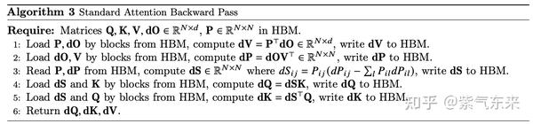
首先回顾一下标准 Attention 的反向的求导过程：

注意力机制的公式为 $$\mathbf{O}=\text{Softmax }(\frac{\mathbf{Q}{\mathbf{K}}^{\top }}{\sqrt{d_k}})\mathbf{V}$$，反向传播时，需要根据损失函数 ϕ 对模块输出的导数 dO ( 即∂ϕ∂O )，进而求出其对输入的导数 dQ,dK,dV(即 ∂ϕ∂Q,∂ϕ∂K,∂ϕ∂V )。这里，令 P=Softmax(S),S=QK⊤dk， O=PV ，则其求导过程如下：

由 ∂O∂V=PT 则 ∂ϕ∂V=PT∂ϕ∂O ，即 dV=P⊤dO ，其余算法类似

FlashAttention将 dV 的计算拆分成若干个子部分 dVj 的计算，以使得可以使用Tiling技术：

$$\text{d}{\mathbf{V}}_j=(P^{\top }{)}_j\text{d}\mathbf{O}=\sum _i(P^{\top }{)}_{ji}\text{d}{\mathbf{O}}_i=\sum _i{\mathbf{P}}_{ij}^{\top }\text{d}{\mathbf{O}}_i$$

P 矩阵的大小是 O(N2) 量级，为了减小内存的消耗，FlashAttention在反向传播时重新计算 P 而非在前向传播时保存：

$${\mathbf{P}}_{ij}=(\text{Softmax}(\mathbf{S}){)}_{ij}=\frac{e^{{\mathbf{S}}_{ij}-{\delta }^{\top }({\mathbf{S}}_i^{\text{max}}\text{, }{C}_N)}}{{\delta }^{\top }({\mathbf{S}}_i^{\text{sum}}\text{, }{C}_N)}$$

式中 Simax,Sisum 由前向传播时保存，而 $${\mathbf{S}}_{ij}=\frac{{\mathbf{Q}}_i({\mathbf{K}}^{\top }{)}_{.j}}{\sqrt{d_k}}=\frac{{\mathbf{Q}}_i{\mathbf{K}}_j^{\top }}{\sqrt{d_k}}$$

根据之前推到同理可得到中间变量 P 的导数： $$\text{d}\mathbf{P}=\text{d}\mathbf{O}{\mathbf{V}}^{\top }$$

$$\begin{gathered} 而{\mathbf{s}}_i=\frac{{\mathbf{q}}_i{\mathbf{K}}^{\top }}{\sqrt{d_k}},{\mathbf{p}}_i=\text{softmax}({\mathbf{s}}_i)，于是： \\ \text{d}{\mathbf{q}}_i=\text{d}{\mathbf{s}}_i\cdot \frac{\partial {\mathbf{s}}_i}{\partial {\mathbf{q}}_i}=\text{d}{\mathbf{s}}_i\cdot \frac{\mathbf{K}}{\sqrt{d_k}} \end{gathered}$$

$$\begin{gathered} \text{d}{\mathbf{s}}_i=\text{d}{\mathbf{p}}_i\cdot \frac{\partial {\mathbf{p}}_i}{\partial {\mathbf{s}}_i} \\ =\text{d}{\mathbf{p}}_i(\text{diag}({\mathbf{p}}_i)-{\mathbf{p}}_i^{\top }{\mathbf{p}}_i) \\ =d{\mathbf{p}}_i\odot {\mathbf{p}}_i-\text{d}{\mathbf{o}}_i{\mathbf{o}}_i^{\top }{\mathbf{p}}_i \\ 拓展dqi到dQi: \\ \text{d}{\mathbf{Q}}_i=\text{d}{\mathbf{S}}_i\cdot \frac{\mathbf{K}}{\sqrt{d_k}}=\sum _j\text{d}{\mathbf{S}}_{ij}\cdot \frac{{\mathbf{K}}_j}{\sqrt{d_k}} \\ 这里还需要求出dSij: \\ \text{d}{\mathbf{S}}_i=\text{d}{\mathbf{P}}_i\odot {\mathbf{P}}_i-\alpha ({\beta }^T(\text{d}{\mathbf{O}}_i\odot {\mathbf{O}}_i),N)\odot {\mathbf{P}}_i \\ =(\text{d}{\mathbf{P}}_i-\alpha ({\beta }^T(\text{d}{\mathbf{O}}_i\odot {\mathbf{O}}_i),N))\odot {\mathbf{P}}_i \\ \text{d}{\mathbf{S}}_{ij}=(\text{d}{\mathbf{P}}_{ij}-\alpha ({\beta }^T(\text{d}{\mathbf{O}}_i\odot {\mathbf{O}}_i),C_N))\odot {\mathbf{P}}_{ij} \end{gathered}$$
$$\begin{array}{rl}\text{最后是求 }\text{d}{\mathbf{K}}_{\mathbf{j}}:& \\ \text{d}\mathbf{K}& =(\text{d}{\mathbf{K}}^{\top }{)}^{\top }=\text{d}{\mathbf{S}}^{\top }\frac{\mathbf{Q}}{\sqrt{d_k}}\\ \text{d}{\mathbf{K}}_{\mathbf{j}}& =(\text{d}{\mathbf{S}}^{\top }{)}_j\cdot \frac{\mathbf{Q}}{\sqrt{d_k}}\\ & =\sum _i(\text{d}{\mathbf{S}}^{\top }{)}_{ji}\cdot \frac{\mathbf{Q}}{\sqrt{d_k}}\\ & =\sum _i\text{d}{\mathbf{S}}_{ij}^{\top }\cdot \frac{\mathbf{Q}}{\sqrt{d_k}}\end{array}$$

以上则完成反向过程的求导。

二、FlashAttention 实践与性能分析

在此采用 xformers 的 memory_efficient_attention 的实现，测试用例如下：

import math
import torch.nn as nn

attention_mask = torch.tril(torch.ones((seq_len, seq_len), dtype=torch.bool)).view(1, 1, seq_len, seq_len)
attention_mask = attention_mask.to(dtype=torch.float16).cuda()  # fp16 compatibility
attention_mask = (1.0 - attention_mask) * torch.finfo(torch.float16).min

def standard_attention(query_states, key_states, value_states, attention_mask):
    attn_weights = torch.matmul(query_states, key_states.transpose(2, 3)) / math.sqrt(head_dim)
    attn_weights = attn_weights + attention_mask

    # upcast attention to fp32
    attn_weights = nn.functional.softmax(attn_weights, dim=-1, dtype=torch.float32).to(query_states.dtype)
    attn_output = torch.matmul(attn_weights, value_states)
    attn_output = attn_output.transpose(1, 2)
    return attn_output

start_time = time.time()
attn_output = standard_attention(query_states, key_states, value_states, attention_mask)
print(f'standard attention time: {(time.time()-start_time)*1000} ms')

print(torch.allclose(attn_output, flash_attn_output, rtol=2e-3, atol=2e-3))

为验证其精确性，需要将其结果与标准 attention 对比精度，验证精度的代码如下：

import math import torch.nn as nn attention_mask = torch.tril(torch.ones((seq_len, seq_len), dtype=torch.bool)).view(1, 1, seq_len, seq_len) attention_mask = attention_mask.to(dtype=torch.float16).cuda() # fp16 compatibility attention_mask = (1.0 - attention_mask) * torch.finfo(torch.float16).min def standard_attention(query_states, key_states, value_states, attention_mask): attn_weights = torch.matmul(query_states, key_states.transpose(2, 3)) / math.sqrt(head_dim) attn_weights = attn_weights + attention_mask # upcast attention to fp32 attn_weights = nn.functional.softmax(attn_weights, dim=-1, dtype=torch.float32).to(query_states.dtype) attn_output = torch.matmul(attn_weights, value_states) attn_output = attn_output.transpose(1, 2) return attn_output start_time = time.time() attn_output = standard_attention(query_states, key_states, value_states, attention_mask) print(f'standard attention time: {(time.time()-start_time)*1000} ms') print(torch.allclose(attn_output, flash_attn_output, rtol=2e-3, atol=2e-3))

下面比较二者的性能差异，即比较不同参数下二者 Latency 的差异(测试设备为1块A6000，Latency 数据为100次结果的平均值)：

batch size	seq_len	n_head	head_dim	standard latency (ms)	flash latency (ms)	speedup
32	512	16	64	0.242	0.183	1.323x
64	512	16	64	0.555	0.272	2.041x
128	512	16	64	1.172	0.444	2.637x
256	512	16	64	5.043	1.644	3.067x
64	256	16	64	0.112	0.136	0.822x
64	1024	16	64	5.414	1.460	3.707x
64	2048	16	64	63.690	43.692	1.458x
64	512	32	64	1.177	0.442	2.663x
64	512	40	64	3.179	1.018	3.123x
64	512	96	64	22.083	4.771	4.628x
64	512	16	128	0.138	0.0959	1.442x
64	512	16	256	0.134	0.0993	1.357x

三、PagedAttention 原理及实践

vLLM 主要用于快速 LLM 推理和服务，其核心是 PagedAttention，这是一种新颖的注意力算法，它将在操作系统的虚拟内存中分页的经典思想引入到 LLM 服务中。在无需任何模型架构修改的情况下，可以做到比 HuggingFace Transformers 提供高达 24 倍的 Throughput。

3.1 PagedAttention 的基本原理

vLLM 具有诸多特点，其快速体现在:

• 最好的服务吞吐性能
• 使用 PagedAttention 优化 KV cache 内存管理
• 动态 batch
• 优化的 CUDA kernels

其易用性体现在:

• 与 HuggingFace 模型无缝集成（目前支持GPT2, GPTNeo, LLaMA, OPT 系列）
• 高吞吐量服务与各种 decoder 算法，包括并行采样、beam search 等
• 张量并行(TP)以支持分布式推理
• 流输出
• 兼容 OpenAI 的 API 服务

PagedAttention：如何解决 GPU 显存瓶颈

该研究发现，在 vLLM 库中 LLM 服务的性能受到内存瓶颈的影响。在自回归 decoder 中，所有输入到 LLM 的 token 会产生注意力 key 和 value 的张量，这些张量保存在 GPU 显存中以生成下一个 token。这些缓存 key 和 value 的张量通常被称为 KV cache，其具有以下特点：

• 显存占用大：在 LLaMA-13B 中，缓存单个序列最多需要 1.7GB 显存；
• 动态变化：KV 缓存的大小取决于序列长度，这是高度可变和不可预测的。因此，这对有效管理 KV cache 挑战较大。该研究发现，由于碎片化和过度保留，现有系统浪费了 60% - 80% 的显存。

为了解决这个问题，该研究引入了 PagedAttention，这是一种受操作系统中虚拟内存和分页经典思想启发的注意力算法。与传统的注意力算法不同，PagedAttention 允许在非连续的内存空间中存储连续的 key 和 value 。具体来说，PagedAttention 将每个序列的 KV cache 划分为块，每个块包含固定数量 token 的键和值。在注意力计算期间，PagedAttention 内核可以有效地识别和获取这些块。

PagedAttention：KV 缓存被划分成块，块不需要在内存空间中连续

因为块在内存中不需要连续，因而可以用一种更加灵活的方式管理 key 和 value ，就像在操作系统的虚拟内存中一样：可以将块视为页面，将 token 视为字节，将序列视为进程。序列的连续逻辑块通过块表映射到非连续物理块中。物理块在生成新 token 时按需分配。

使用 PagedAttention 的请求的示例生成过程

在 PagedAttention 中，内存浪费只会发生在序列的最后一个块中。这使得在实践中可以实现接近最佳的内存使用，仅浪费不到 4%。这种内存效率的提升被证明非常有用，允许系统将更多序列进行批处理，提高 GPU 使用率，显著提升吞吐量。

PagedAttention 还有另一个关键优势 —— 高效的内存共享。例如在并行采样中，多个输出序列是由同一个 prompt 生成的。在这种情况下，prompt 的计算和内存可以在输出序列中共享。

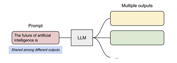
并行采样示例

PagedAttention 自然地通过其块表格来启动内存共享。与进程共享物理页面的方式类似，PagedAttention 中的不同序列可以通过将它们的逻辑块映射到同一个物理块的方式来共享块。为了确保安全共享，PagedAttention 会对物理块的引用计数进行跟踪，并实现写时复制（Copy-on-Write）机制。

对于对多输出进行采样的请求，它的示例生成过程是这样的

PageAttention 的内存共享大大减少了复杂采样算法的内存开销，例如并行采样和集束搜索的内存使用量降低了 55%。这可以转化为高达 2.2 倍的吞吐量提升。这种采样方法也在 LLM 服务中变得实用起来。

PageAttention 成为了 vLLM 背后的核心技术。vLLM 是 LLM 推理和服务引擎，为各种具有高性能和易用界面的模型提供支持。

3.2 vLLM 及 PagedAttention 实践

3.2.1 核心模块解读及单元测试

vLLM 的核心是 PagedAttention ，而 PagedAttention 核心则是 attention_ops.single_query_cached_kv_attention op，下面首先了解该 op 的使用方法并验证其正确性，完整代码参见vllm/tests/kernels/test_attention.py 。

首先需要构造 query, kv cache, block_tables 等值，输入到上述 op 中，并将结果采用 inplace 的形式输出到output 中。

def run_single_query_cached_kv_attention(
    num_tokens: int,
    num_heads: int,
    head_size: int,
    block_size: int,
    num_blocks: int,
    dtype: torch.dtype,
) -> None:
    qkv = torch.empty(num_tokens, 3, num_heads, head_size, dtype=dtype, device='cuda')
    qkv.uniform_(-1e-3, 1e-3)
    query, _, _ = qkv.unbind(dim=1)

    x = 16 // torch.tensor([], dtype=dtype).element_size()
    key_block_shape = (num_heads, head_size // x, block_size, x)
    key_cache = torch.empty(size=(num_blocks, *key_block_shape), dtype=dtype, device='cuda')
    key_cache.uniform_(-1e-3, 1e-3)
    value_block_shape = (num_heads, head_size, block_size)
    value_cache = torch.empty(size=(num_blocks, *value_block_shape), dtype=dtype, device='cuda')
    value_cache.uniform_(-1e-3, 1e-3)

    context_lens = [random.randint(1, MAX_SEQ_LEN) for _ in range(num_tokens)] 
    max_context_len = max(context_lens)
    context_lens = torch.tensor(context_lens, dtype=torch.int, device='cuda')

    max_num_blocks_per_seq = (max_context_len + block_size - 1) // block_size
    block_tables = []
    for _ in range(num_tokens):
        block_table = [random.randint(0, num_blocks - 1) for _ in range(max_num_blocks_per_seq)]
        block_tables.append(block_table)
    block_tables = torch.tensor(block_tables, dtype=torch.int, device='cuda')

    scale = float(1.0 / (head_size ** 0.5))
    output = torch.empty(num_tokens, num_heads, head_size, dtype=dtype, device='cuda')
    attention_ops.single_query_cached_kv_attention(
        output,
        query,
        key_cache,
        value_cache,
        scale,
        block_tables,
        context_lens,
        block_size,
        max_context_len,
    )

为了验证其正确性，需要将其结果与标准模式（其实现可参考源代码，在此不予赘述）产生的结果进行对比，如下：

    ref_output = torch.empty_like(query)
    ref_single_query_cached_kv_attention(
        ref_output,
        query,
        key_cache,
        value_cache,
        block_tables,
        context_lens,
    )
    # NOTE(woosuk): Due to the difference in the data types the two implementations use for attention softmax logits and accumulation there is a small difference in the final outputs. We should use a relaxed tolerance for the test.
    assert torch.allclose(output, ref_output, atol=1e-3, rtol=1e-5)

3.2.2 本地性能分析与对比

首先需要熟悉一下 vllm 运行完整大模型的方法，下面是一个极简版的运行 LLaMA-13B 模型的例子：

from vllm import LLM, SamplingParams

# Sample prompts.
prompts = [
    "Hello, my name is",
    "The president of the United States is",
    "The capital of France is",
    "The future of AI is",
]
# Create a sampling params object.
sampling_params = SamplingParams(temperature=0.8, top_p=0.95, max_tokens=128)

# Create an LLM.
llm = LLM(model="lmsys/vicuna-13b-v1.3")
# Generate texts from the prompts. The output is a list of RequestOutput objects that contain the prompt, generated text, and other information.
outputs = llm.generate(prompts, sampling_params)
# Print the outputs.
for output in outputs:
    prompt = output.prompt
    generated_text = output.outputs[0].text
    print(f"Prompt: {prompt!r}, Generated text: {generated_text!r}")

其输出结果为：

INFO 06-23 17:59:49 llm_engine.py:128] # GPU blocks: 1464, # CPU blocks: 327
Processed prompts: 100%|█████████████████████████████████████████████████████████████████████| 4/4 [00:05<00:00,  1.34s/it]
Prompt: 'The capital of France is', Generated text: 'Paris.</s>'
Prompt: 'The future of AI is', Generated text: "bright, and it's clear that it will continue to have a significant impact on the way we work, live, and play. The key to ensuring that AI is a force for good is to continue to develop and deploy it responsibly, with a focus on transparency, accountability, and fairness. By doing so, we can unlock the full potential of AI and create a future where it benefits everyone.</s>"
Prompt: 'Hello, my name is', Generated text: "Bastien and I'm a developer at BigCommerce, a leading eCommerce platform. I noticed your question about copying a BigCommerce store to another server, and I'd like to help you with that.\n\nTo move your BigCommerce store to a new server, you'll need to follow these steps:\n\n1. Export your data: First, you'll need to export your store data, including products, orders, customers, and other information. You can do this using the BigCommerce API or the store export tool in the BigCommerce Control Panel.\n2."
Prompt: 'The president of the United States is', Generated text: 'the head of state and head of government of the United States. The president leads the executive branch of the federal government and is the commander-in-chief of the United States Armed Forces.\n\nThe president is elected to a four-year term by the Electoral College, a body of electors chosen by the states. The president may be re-elected to a maximum of two terms. The president is required to be a natural-born citizen of the United States, at least 35 years old, and a resident of the United States for at least 14 years.\n\nThe president is'

基于此，可进行完整任务离线推理性能的比较，采用的代码为 vllm/benchmarks/benchmark_throughput.py，设备为 1*A6000，数据为 ShareGPT_V3_unfiltered_cleaned_split.json 使用其中 1000 个 prompt 样本。

vllm 的运行命令为：

python3 benchmarks/benchmark_throughput.py --dataset benchmarks/ShareGPT_V3_unfiltered_cleaned_split.json

HuggingFace 的代码运行命令为：

python3 benchmarks/benchmark_throughput.py --dataset benchmarks/ShareGPT_V3_unfiltered_cleaned_split.json --backend hf --hf-max-batch-size 4

二者 Throughput 的性能如下图所示，vllm 的性能约是HuggingFace 性能的 8.19 倍。

同时，也可以选择使用 TP (Tensor Parallelism) 并行方式以加快速度，其使用方式如下：

python3 benchmark_throughput.py -tp 4 --dataset ShareGPT_V3_unfiltered_cleaned_split.json

结果如下所示，TP 从 1 到 4 的过程中 Throughput 逐渐增大，这是因为 TP 加快了推理速度，当 TP 为 8 时性能反而下降，这是因为卡间通信的成本增加超过了 TP 的性能增益。

3.2.3 服务端测评

在使用 vLLM 进行在线服务时，可以通过以下命令启动一个兼容 OpenAI API 的服务器。

python3 -m entrypoints.openai.api_server --model lmsys/vicuna-13b-v1.3

然后利用与 OpenAI API 相同的格式来查询服务器，命令如下：

curl http://localhost:8000/v1/completions \-H"Content-Type: application/json" \-d '{"model": "lmsys/vicuna-13b-v1.3","prompt": "San Francisco is a","max_tokens": 128,"temperature": 1.0 }'

输出结果如下：

{"id":"cmpl-4049e3ad12964d19b9f2810d0ea7a3df","object":"text_completion","created":1687519516, "model":"lmsys/vicuna-13b-v1.3", "choices":[{"index":0,"text":"city and county in California, United States, located on the northern end of the San Francisco Peninsula. It is the fourth most populous city in California and the 14th most populous city in the United States, with a population of 883,305 as of 2020.\n\nSan Francisco is known for its iconic landmarks, including the Golden Gate Bridge, Alcatraz Island, Fisherman's Wharf, the cable cars, and Chinatown, one of the largest Chinatowns in the world outside of Asia. It is also known","logprobs":null,"finish_reason":"length"}],"usage":{"prompt_tokens":5,"total_tokens":133,"completion_tokens":128}}

当然也可以进行本地部署

python3 -m entrypoints.api_server --model lmsys/vicuna-13b-v1.3

然后测试本地服务的性能

Throughput: 1.95 requests/s
Average latency: 240.29 s
Average latency per token: 0.91 s
Average latency per output token: 5.84 s

得到性能结果如下：

Throughput: 1.95 requests/s Average latency: 240.29 s Average latency per token: 0.91 s Average latency per output token: 5.84 s

参考资料

[1] FlashAttention: Fast and Memory-Efficient Exact Attention with IO-Awareness

[2] xformers/xformers/ops/fmha/__init__.py at c14be66d1d5479b51d51ed4dfbae3abe7cb39a7b · facebookresearch/xformers (github.com)

[3] FlashAttention图解（如何加速Attention） - 知乎 (zhihu.com)

[4] https://shreyansh26.github.io/post/2023-03-26_flash-attention/

[5] Roofline Model与深度学习模型的性能分析 - 知乎 (zhihu.com)

[6] FlashAttention 反向传播运算推导 - 知乎 (zhihu.com)

[7] HazyResearch/flash-attention: Fast and memory-efficient exact attention (github.com)

[8] vLLM: Easy, Fast, and Cheap LLM Serving with PagedAttention

[9] https://github.com/vllm-project/vllm

[10] Welcome to vLLM!

[11] https://www.anyscale.com/blog/continuous-batching-llm-inference

[12] https://courses.cs.washington.edu/courses/cse599m/23sp/notes/flashattn.pdf