用Mathematica生成一系列具有类似分形特征的曲线

最新推荐文章于 2024-06-10 21:38:37 发布

stereohomology

最新推荐文章于 2024-06-10 21:38:37 发布

阅读量3.3k

点赞数 1

分类专栏：学习学习文章标签： mathematica 迭代

学习学习专栏收录该内容

670 篇文章 14 订阅

订阅专栏

来源

Two-dimensional L-systems

此外，可以参考Stan Wagon的：
Mathematica in Action: Problem solving through visualization （3rd Edition by Springer 2010）一书及其代码。

描述和基本代码

（摘要）定义系列的符号规则，然后迭代……差不多就是复杂的分形。

L-systems (also called Lindenmayer systems or parallel string-rewrite systems) are a compact way to describe iterative graphics using a turtle analogy, similar to that used by the LOGO programming language (about which I know nothing).

An L-system is created by starting with an axiom, such as a line segment, and one or more production rules, which are statements such as “replace every line segment with a left turn, a line segment, a right turn, another segment…”. When this system is iterated several times, the result is often a complicated fractal curve.

When programming L-systems, one typically represents the axiom as a sequence of characters, such as $F$ , and the production rules as replacement rules of the form $F -> F+F--F+F$ . We then carry out the string replacements (in parallel) as many times as desired. For example, we iterate the axiom and production rule just described in the following way:

We start with the axiom F, and replace every occurrence of F with $F+F--F+F$ , resulting in the string

$F+F--F+F$ .

We then replace every occurrence of F in the result with $F+F--F+F$ , resulting in the string

$F+F--F+F+F+F--F+F--F+F--F+F+F+F--F+F$ .

Carrying out the replacement one more time results in the following:

$F+F--F+F+F+F--F+F--F+F--F+F+F+F--F+F+F+F--F+F+F+F--F+F--F+F--F+F+F+F--F+F-- F+F--F+F+F+F--F+F--F+F--F+F+F+F--F+F+F+F--F+F+F+F--F+F--F+F--F+F+F+F--F+F$ .

After the desired number of iterations has been carried out, we render the L-system string using the turtle analogy. A typical interpretation of our string is that an F is an instruction to draw a line segment one unit in the current direction, a + is an instruction to rotate the current direction one angular unit clockwise, and a - is an instruction to rotate the current direction one angular unit counterclockwise. (Other characters and interpretations are of course up to us.) If we assume for this example that one (angular) unit is Pi/3 radians, the following are the partial results (omitting the zeroth iteration, the axiom).

这里基本代码可以放在m文件中；直接在notebook中也能用。

(* carry out the forward and backward moves and the various
    rotations by updating the global location 'Lpos' and
    direction angle 'Ltheta'. *)

Lmove[ z_String, Ldelta_ ] :=
    Switch[ z,
        "+", Ltheta += Ldelta;,
        "-", Ltheta -= Ldelta;,
        "F", Lpos += {Cos[Ltheta], Sin[Ltheta]},
        "B", Lpos -= {Cos[Ltheta], Sin[Ltheta]},
         _ , Lpos += 0. ];

LSystem::usage =
    "LSystem[axiom, {rules}, n, Ldelta:90 Degree]
    creates the L-string for the nth iteration of
    the list 'rules', starting with the string 'axiom'.";

(* make the string: starting with 'axiom', use StringReplace the specified number of times *)

LSystem[ axiom_, rules_List,
    n_Integer, Ldelta_:N[90 Degree]] :=

    Nest[ StringReplace[#, rules]&, axiom, n ];

Off[General::spell1];

(* initialize the position 'Lpos' and the direction angle 'Ltheta';     create the Line graphics primitive represented by the L-system by mapping 'Lmove' over the characters in the L-string, deleting all the
    Nulls; then show the Graphics object *)

LShow[lstring_String, Ldelta_:N[90 Degree]] :=
   (Lpos={0.,0.};
    Ltheta=0.;
    Show[
      Graphics[Line[
        Prepend[
          DeleteCases[
            Map[Lmove[#, Ldelta]&, Characters[lstring]],
           Null ],
        {0,0}]]],
     AspectRatio -> Automatic]);

(*same as above, plus a list of colors for each segment contained in  'templist' -- unfortunately, 'templist' isn't really 'temp', but  stays in memory as a global variable; so sue me *)

LShowColor[lstring_String, Ldelta_:N[90 Degree]] :=
   (Lpos = {0., 0.};
    Ltheta = 0.;

    templist =
      Map[ Line,
        Partition[
          Prepend[
            DeleteCases[
              Map[ Lmove[#, Ldelta]&, Characters[lstring] ],
             Null],
           {0,0}],
         2,1]];

    ncol = N[Length[templist]];

    huelist = Table[ Hue[k/ncol], {k, 1., ncol} ];

    Show[
      Graphics[
        N[Flatten[Transpose[{huelist, templist}]]]],
     AspectRatio -> Automatic]);

On[General::spell1];

例子

下面这些代码利用前面的基本代码，可以生成不同的分形曲线：

LShowColor[(*Koch curve*)LSystem["F", {"F" -> "F+F--F+F"}, 6],  N[60 Degree]]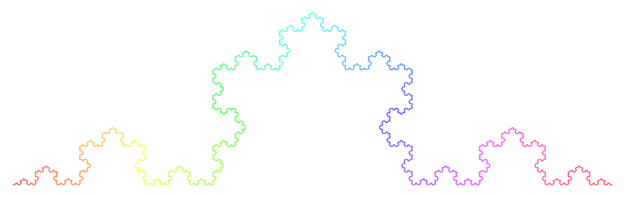

这里写图片描述

LShowColor[(*Peano curve 皮亚诺曲线*)
  LSystem["F", {"F" -> "F+F-F-F-F+F+F+F-F"}, 4]]

这里写图片描述

LShowColor[(*Quadratic Koch island *)
  LSystem["F+F+F+F", {"F" -> "F-F+F+FFF-F-F+F"}, 3]]

LShowColor[(*32-segment curve*)
  LSystem["F+F+F+F", {"F" -> 
     "-F+F-F-F+F+FF-F+F+FF+F-F-FF+FF-FF+F+F-FF-F-F+FF-F-F+F+F-F+"}, 
   2]]

LShowColor[
  LSystem["YF",(*Sierpinski arrowhead*){"X" -> "YF+XF+Y",  "Y" -> "XF-YF-X"}, 7], N[60 Degree]]

LShowColor[(*Peano-Gosper curve*)
  LSystem["FX", {"X" -> "X+YF++YF-FX--FXFX-YF+", 
    "Y" -> "-FX+YFYF++YF+FX--FX-Y"}, 4], N[60 Degree]]

LShowColor[(*Sierpinski triangle*)
  LSystem["FXF--FF--FF", {"F" -> "FF", "X" -> "--FXF++FXF++FXF--"}, 6], N[60 Degree]]

LShowColor@
  LSystem["F+XF+F+XF",(*Square curve*){"X" -> "XF-F+F-XF+F+XF-F+F-X"},4]

LShowColor[(*Dragon curve*)
  LSystem["FX", {"X" -> "X+YF+", "Y" -> "-FX-Y"}, 12]]

LShowColor@
  LSystem["L",(*Hilbert curve我是找希尔伯特曲线的生成代码时发现这个帖子的*){"L" -> "+RF-LFL-FR+", "R" -> "-LF+RFR+FL-"}, 6]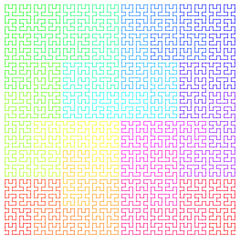

这里写图片描述

LShowColor@
  LSystem["X",(*Hilbert curve II*){"X" -> "XFYFX+F+YFXFY-F-XFYFX", "Y" -> "YFXFY-F-XFYFX+F+YFXFY"}, 3]

三维版本：

Off[General::spell1, General::spell];

(*the 3D rotation matrices*)

RotMatPsi[
   angle_] := {{Cos[angle], Sin[angle], 0}, {-Sin[angle], Cos[angle], 
    0}, {0, 0, 1}};

RotMatPsiII[
   angle_] := {{Cos[angle], -Sin[angle], 0}, {Sin[angle], Cos[angle], 
    0}, {0, 0, 1}};

RotMatTheta[
   angle_] := {{Cos[angle], 0, Sin[angle]}, {0, 1, 0}, {-Sin[angle], 
    0, Cos[angle]}};

RotMatThetaII[
   angle_] := {{Cos[angle], 0, -Sin[angle]}, {0, 1, 0}, {Sin[angle], 
    0, Cos[angle]}};

RotMatPhi[
   angle_] := {{1, 0, 0}, {0, Cos[angle], 
    Sin[angle]}, {0, -Sin[angle], Cos[angle]}};

RotMatPhiII[
   angle_] := {{1, 0, 0}, {0, Cos[angle], -Sin[angle]}, {0, 
    Sin[angle], Cos[angle]}};

On[General::spell1, General::spell];

(*make the string:starting with'axiom',use StringReplace the \
specified number of times*)

LSystem[axiom_, rules_List, n_Integer, 
   Ldelta_: {N[90 Degree], N[90 Degree], N[90 Degree]}] := 
  Nest[StringReplace[#, rules] &, axiom, n];

(*carry out the forward and backward moves and the various 3D \
rotations by updating the global location'Lpos' and direction \
matrix'Ldir'.*)

Lmove[z_String, Ldelta_] := 
  Switch[z, "F", Lpos += First[Transpose[Ldir]], "B", 
   Lpos -= First[Transpose[Ldir]], "+", 
   Ldir = Ldir.RotMatPsi[Ldelta[[1]]];, "-", 
   Ldir = Ldir.RotMatPsiII[Ldelta[[1]]];, "^", 
   Ldir = Ldir.RotMatTheta[Ldelta[[2]]];, "&", 
   Ldir = Ldir.RotMatThetaII[Ldelta[[2]]];, "<", 
   Ldir = Ldir.RotMatPhi[Ldelta[[3]]];, ">", 
   Ldir = Ldir.RotMatPhiII[Ldelta[[3]]];, _, Null];

(*initialize the position'Lpos' and the direction matrix'Ldir';
create the Line graphics primitive represented by the L-system by \
mapping'Lmove' over the characters in the L-string,deleting all the \
Nulls;then show the Graphics3D object*)

LShow3D[lstring_String, 
   Ldelta_: {N[90 Degree], N[90 Degree], 
     N[90 Degree]}] := (Lpos = {0., 0., 0.};
   Ldir = N[IdentityMatrix[3]];
   Show[Graphics3D[
     Line[Prepend[
       DeleteCases[(Lmove[#, Ldelta] &) /@ Characters[lstring], 
        Null], {0, 0, 0}]]], AspectRatio -> Automatic]);

(*same as above,plus a list of colors for each segment contained \
in'templist'-- unfortunately,'templist' isn't really'temp',but stays \
in memory as a global variable;so sue me*)

LShowColor3D[lstring_String, 
   Ldelta_: {N[90 Degree], N[90 Degree], N[90 Degree]}, 
   opts___Rule] := (Lpos = {0., 0., 0.};
   Ldir = 
    N[IdentityMatrix[3]] templist = 
     Line /@ Partition[
       Prepend[DeleteCases[(Lmove[#, Ldelta] &) /@ 
          Characters[lstring], Null], {0, 0, 0}], 2, 1];
   ncol = N[Length[templist]];
   huelist = Table[Hue[k/ncol], {k, 1., ncol}];
   Show[Graphics3D[N[Flatten[Transpose[{huelist, templist}]]]], 
    AspectRatio -> Automatic, opts]);

(*create just the list of 3D corners,supposing such a thing desirable*)

LCorners3D[lstring_String, 
   Ldelta_: {N[90 Degree], N[90 Degree], 
     N[90 Degree]}] := (Lpos = {0., 0., 0.};
   Ldir = N[IdentityMatrix[3]];
   Prepend[
    DeleteCases[(Lmove[#, Ldelta] &) /@ Characters[lstring], 
     Null], {0, 0, 0}]);

(*code for the colored-line version of the Hilbert curve*)

LShowColor3D[
  LSystem["X", {"X" -> "^<XF^<XFX-F^>>XFX&F+>>XFX-F>X->"}, 4], 
  Pi/2.0 {1, 1, 1}, Boxed -> False];

stereohomology

关注

1
点赞
踩
3

收藏

觉得还不错? 一键收藏
0
评论
用Mathematica生成一系列具有类似分形特征的曲线

来源Two-dimensional L-systems此外，可以参考Stan Wagon的： Mathematica in Action: Problem solving through visualization （3rd Edition by Springer 2010）一书及其代码。描述和基本代码（摘要）定义系列的符号规则，然后迭代……差不多就是复杂的分形。L-systems (also c
复制链接

扫一扫