机器学习实践三---神经网络学习

Neural Networks

在这个练习中，将实现神经网络BP算法,练习的内容是手写数字识别。

Visualizing the data

这次数据还是5000个样本，每个样本是一张20*20的灰度图片

    fig, ax_array = plt.subplots(nrows=10, ncols=10, figsize=(6, 4))
    for row in range(10):
        for column in range(10):
            ax_array[row, column].matshow(sample_images[10 * row + column].reshape((20, 20)).T, cmap='gray')
            ax_array[row, column].axis('off')
    plt.show()
    return


data = loadmat("ex4data1.mat")
X = data['X']
y = data['y']

m = X.shape[0]
rand_sample_num = np.random.permutation(m)
sample_images = X[rand_sample_num[0:100], :]
display_data(sample_images)

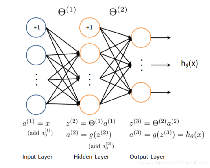
Model representation

这是一个简单的神经网络，输入层、隐藏层、输出，样本图片是20*20，所以输入层是400个单元，（再加上一个额外偏差单元），第二层隐藏层是25个单元， 输出层是10个单元。从上面的数据显示中有两个变量X 和y。
ex4weights.mat 中提供了训练好的网络参数theta1, theta2,
theta1 has size 25 x 401
theta2 has size 10 x 26

Feedforward and cost function

为了最后的输出，我们将标签值也就是数字从0到9， 转化为one-hot 码

from sklearn.preprocessing import OneHotEncoder
def to_one_hot(y):
    encoder =  OneHotEncoder(sparse=False)  # return a array instead of matrix
    y_onehot = encoder.fit_transform(y.reshape(-1,1))
    return y_onehot

加载数据

X, label_y = load_mat('ex4data1.mat')
X = np.insert(X, 0, 1, axis=1)
y = to_one_hot(label_y)

load weight

def load_weight(path):
    data = loadmat(path)
    return data['Theta1'], data['Theta2']

t1, t2 = load_weight('ex4weights.mat')

theta 转化
因为opt.minimize传参问题，我们这里对theta进行平坦化

# 展开
def unrool(var1, var2):
    return np.r_[var1.flatten(), var2.flatten()]
# 分开矩阵化
def rool(array):
    return array[:25*401].reshape(25, 401), array[25*401:].reshape(10, 26)

Feedforward Regularized cost function

这里主要是前馈传播 和 代价函数的一些逻辑，正则化为了预防高方差问题。

def sigmoid(z):
    return 1 / (1 + np.exp(-z))


#前馈传播
def feed_forward(theta, X):
    theta1, theta2 = rool(theta)
    a1 = X
    z2 = a1.dot(theta1.T)
    a2 = np.insert(sigmoid(z2), 0, 1, axis=1)
    z3 = a2.dot(theta2.T)
    a3 = sigmoid(z3)
    return a1, z2, a2, z3, a3

# a1, z2, a2, z3, h = feed_forward(t1, t2, X)


def cost(theta, X, y):
    a1, z2, a2, z3, h = feed_forward(theta, X)
    J = -y * np.log(h) - (1-y) * np.log(1 - h)
    return J

# Implement Regularization
def regularized_cost(theta, X, y, l=1):
    theta1, theta2 = rool(theta)
    temp_theta1 = theta1[:, 1:]
    temp_theta2 = theta2[:, 1:]

    reg = temp_theta1.flatten().T.dot(temp_theta1.flatten()) + temp_theta2.flatten().T.dot(temp_theta2.flatten())
	regularized_theta = l / (2 * len(X)) * reg 
    return regularized_theta + cost(theta, X, y)

Backprogation

反向传播算法，是机器学习比较难推理的算法了， 也是最重要的算法，为了得到最优的theta值， 通过进行反向传播，来不断跟新theta值, 当然还有一些超参数，如lambda、a 、训练迭代次数，如果进行adam、Rmsprop等优化学习效率算法，还有有一些其他的超参数。

# random initalization

# 梯度
def gradient(theta, X, y):
    theta1, theta2 = rool(theta)
    a1, z2, a2, z3, h = feed_forward(theta, X)
    d3 = h - y
    d2 = d3.dot(theta2[:, 1:]) * sigmoid_gradient(z2)
    D2 = d3.T.dot(a2)
    D1 = d2.T.dot(a1)
    D = (1 / len(X)) * unrool(D1, D2)
    return D

Sigmoid gradient

也就是对sigmoid 函数求导

def sigmoid_gradient(z):
    return sigmoid(z) * (1 - sigmoid(z))

Random initialization

初始化参数，我们一般使用随机初始化np.random.randn(-2,2),生成高斯分布，再乘以一个小的数，这样把它初始化为很小的随机数，
这样直观地看就相当于把训练放在了逻辑回归的直线部分进行开始，初始化参数还可以尽量避免梯度消失和梯度爆炸的问题。

def random_init(size):
    return np.random.randn(-2, 2, size) * 0.01

Backporpagation

Regularized Neural Networks

正则化神经网络

def regularized_gradient(theta, X, y, l=1):
    a1, z2, a2, z3, h = feed_forward(theta, X)
    D1, D2 = rool(gradient(theta, X, y))
    t1[:, 0] = 0
    t2[:, 0] = 0
    reg_D1 = D1 + (l / len(X)) * t1
    reg_D2 = D2 + (l / len(X)) * t2
    return unrool(reg_D1, reg_D2)

Learning parameters using fmincg

调优参数

def nn_training(X, y):
    init_theta = random_init(10285)  # 25*401 + 10*26
    res = opt.minimize(fun=regularized_cost,
                       x0=init_theta,
                       args=(X, y, 1),
                       method='TNC',
                       jac=regularized_gradient,
                       options={'maxiter': 400})
    return res

res = nn_training(X, y)

准确率
def accuracy(theta, X, y):
_, _, _, _, h = feed_forward(res.x, X)
y_pred = np.argmax(h, axis=1) + 1
print(classification_report(y, y_pred))

accuracy(res.x, X, label_y)

Visualizing the hidden layer

隐藏层显示跟输入层显示差不多

def plot_hidden(theta):
    t1, _ = rool(theta)
    t1 = t1[:, 1:]
    fig, ax_array = plt.subplots(5, 5, sharex=True, sharey=True, figsize=(6, 6))
    for r in range(5):
        for c in range(5):
            ax_array[r, c].matshow(t1[r * 5 + c].reshape(20, 20), cmap='gray_r')
            plt.xticks([])
            plt.yticks([])
    plt.show()

plot_hidden(res.x)

super parameter lambda update

神经网络是非常强大的模型，可以形成高度复杂的决策边界。如果没有正则化，神经网络就有可能“过度拟合”一个训练集，从而使它在训练集上获得接近100%的准确性，但在以前没有见过的新例子上则不会。你可以设置较小的正则化λ值和MaxIter参数高的迭代次数为自己看到这个结果。