空间单细胞｜Slide-seq分析、可视化与整合(1)

数据集

在本文中，我们将对利用Slide-seq v2技术获得的小鼠海马区数据集进行深入分析。

为了方便数据获取，您可以利用我们的SeuratData包，具体操作示例如下。一旦安装了该数据集，您只需输入?ssHippo，即可查看构建Seurat对象时所使用的命令列表。

InstallData("ssHippo")

slide.seq <- LoadData("ssHippo")

预处理

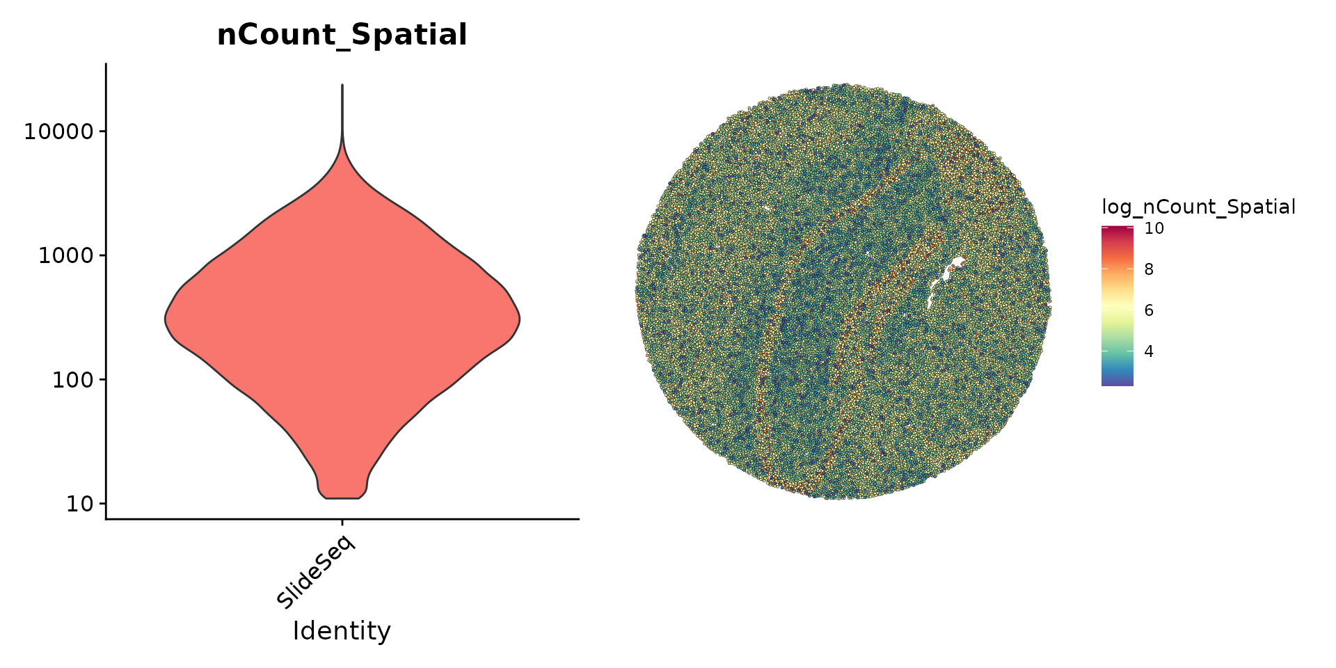
在处理珠子的基因表达数据的初步预处理过程中，我们采用了与其他空间Seurat分析以及常规的单细胞RNA测序实验相似的方法。我们发现，尽管许多珠子的UMI计数非常低，但我们决定保留所有已检测到的珠子，以便进行后续的分析工作。

plot1 <- VlnPlot(slide.seq, features = "nCount_Spatial", pt.size = 0, log = TRUE) + NoLegend()
slide.seq$log_nCount_Spatial <- log(slide.seq$nCount_Spatial)
plot2 <- SpatialFeaturePlot(slide.seq, features = "log_nCount_Spatial") + theme(legend.position = "right")
wrap_plots(plot1, plot2)

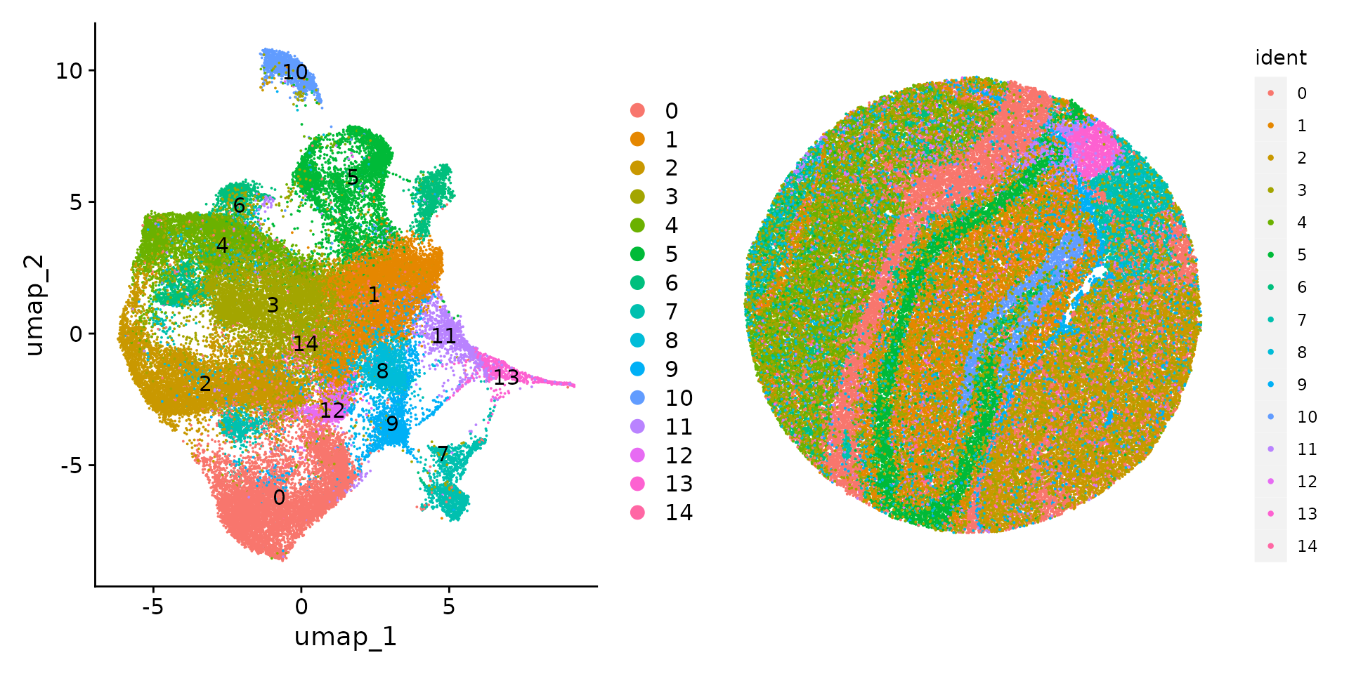
然后，我们使用 sctransform 对数据进行标准化，并执行标准的 scRNA-seq 降维和聚类工作流程。

slide.seq <- SCTransform(slide.seq, assay = "Spatial", ncells = 3000, verbose = FALSE)
slide.seq <- RunPCA(slide.seq)
slide.seq <- RunUMAP(slide.seq, dims = 1:30)
slide.seq <- FindNeighbors(slide.seq, dims = 1:30)
slide.seq <- FindClusters(slide.seq, resolution = 0.3, verbose = FALSE)

然后，我们可以在 UMAP 空间（使用 DimPlot()）或使用 SpatialDimPlot() 在珠坐标空间中可视化聚类结果。

plot1 <- DimPlot(slide.seq, reduction = "umap", label = TRUE)
plot2 <- SpatialDimPlot(slide.seq, stroke = 0)
plot1 + plot2

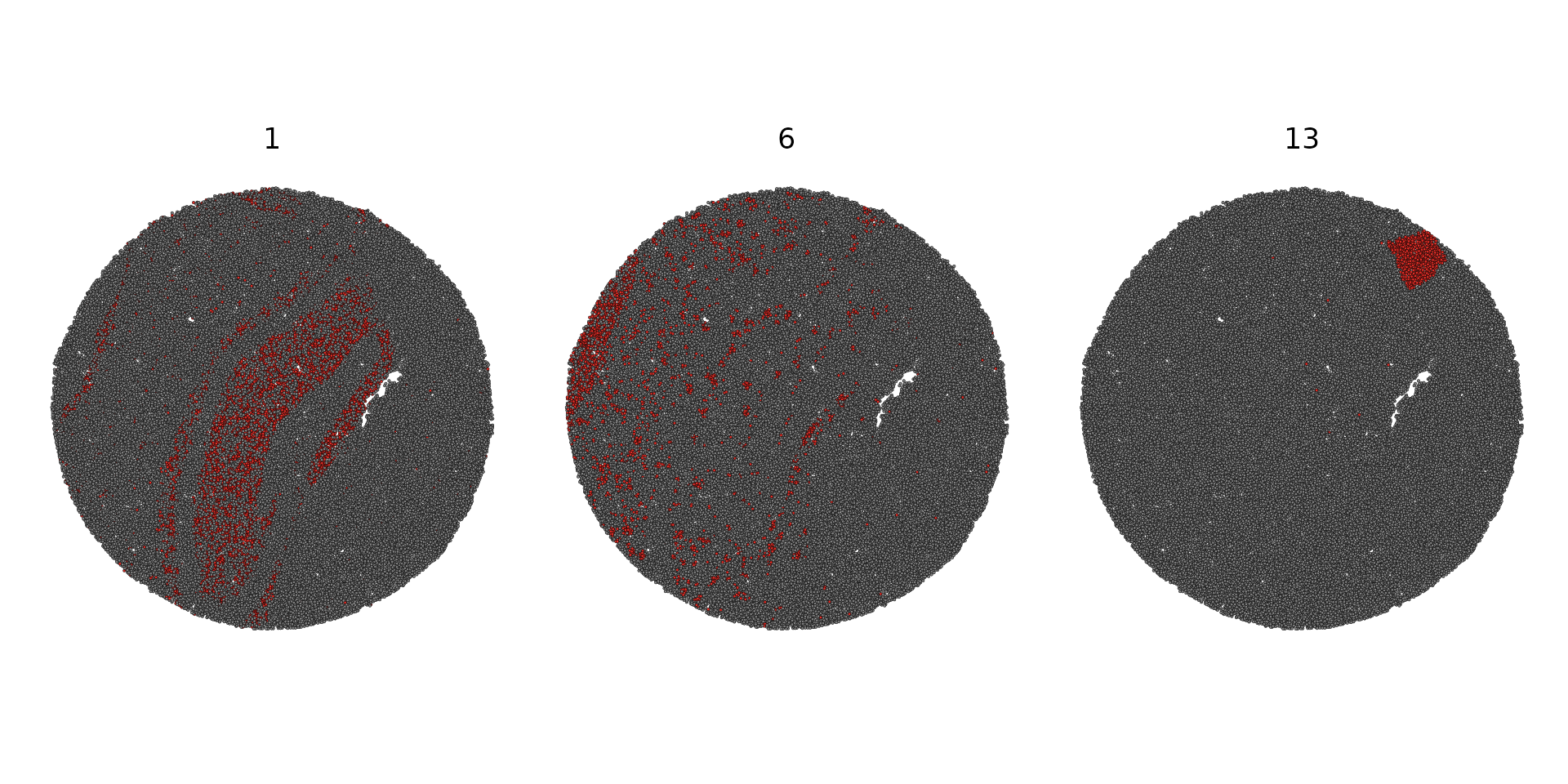
SpatialDimPlot(slide.seq, cells.highlight = CellsByIdentities(object = slide.seq, idents = c(1,
    6, 13)), facet.highlight = TRUE)

与 scRNA-seq 整合

为了方便对Slide-seq数据集进行细胞类型的标注，我们正在使用Saunders和Macosko等人在2018年发表的一个现有小鼠单细胞RNA-seq海马区数据集。

ref <- readRDS("/brahms/shared/vignette-data/mouse_hippocampus_reference.rds")
ref <- UpdateSeuratObject(ref)

文章中提供的原始注释可以在Seurat对象的细胞元数据中找到。这些注释覆盖了多个“分辨率”级别，包括从宽泛的类别（ref subcluster）。我们将基于对细胞类型注释（ref$celltype）的一次调整来进行工作，我们认为这样的调整在保持平衡方面做得很好。

我们将首先执行Seurat的标签转移方法，以此来预测每个珠子的主要细胞类型。

anchors <- FindTransferAnchors(reference = ref, query = slide.seq, normalization.method = "SCT",
    npcs = 50)
predictions.assay <- TransferData(anchorset = anchors, refdata = ref$celltype, prediction.assay = TRUE,
    weight.reduction = slide.seq[["pca"]], dims = 1:50)
slide.seq[["predictions"]] <- predictions.assay

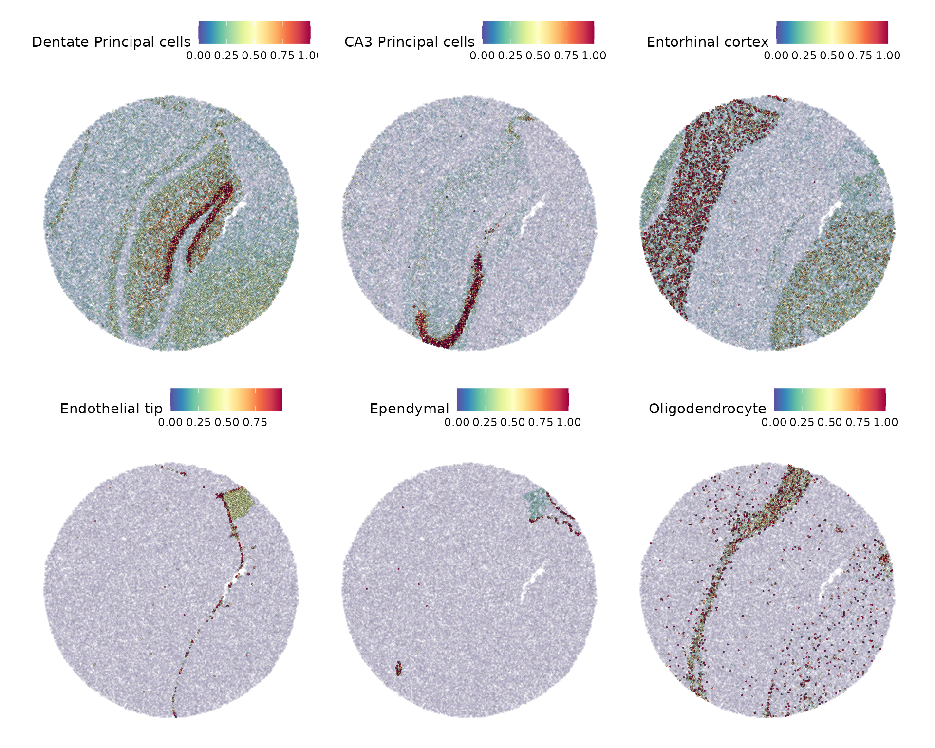
然后我们可以可视化一些主要预期类别的预测分数。

DefaultAssay(slide.seq) <- "predictions"
SpatialFeaturePlot(slide.seq, features = c("Dentate Principal cells", "CA3 Principal cells", "Entorhinal cortex",
    "Endothelial tip", "Ependymal", "Oligodendrocyte"), alpha = c(0.1, 1))

slide.seq$predicted.id <- GetTransferPredictions(slide.seq)
Idents(slide.seq) <- "predicted.id"
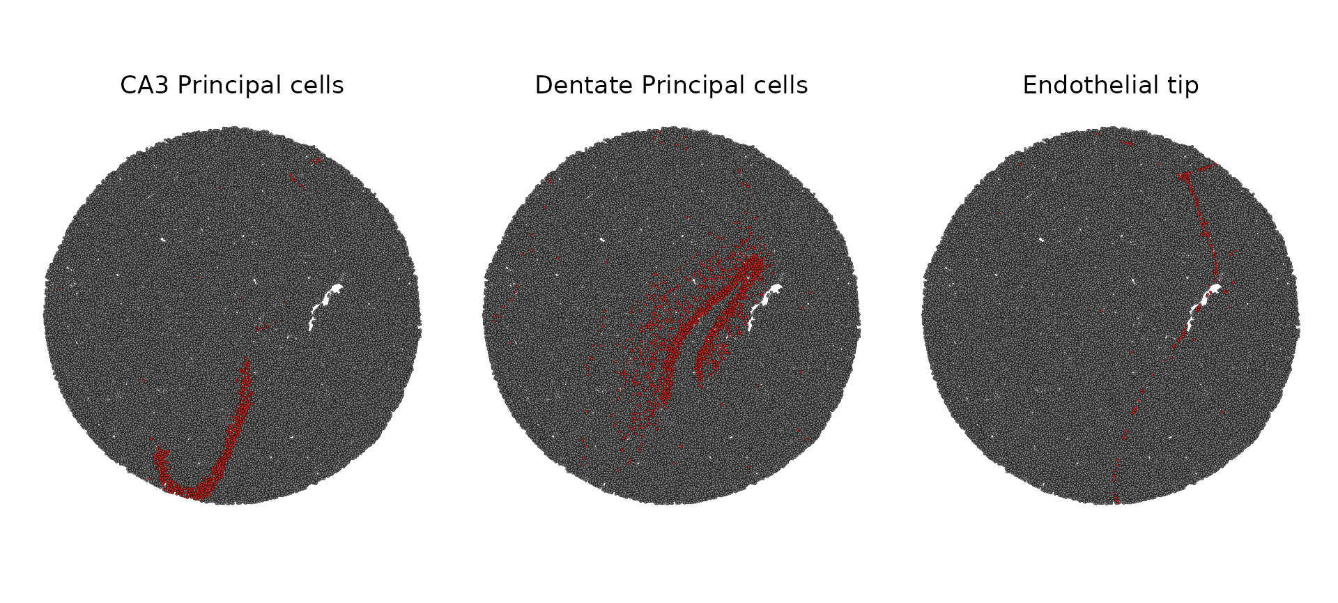
SpatialDimPlot(slide.seq, cells.highlight = CellsByIdentities(object = slide.seq, idents = c("CA3 Principal cells",
    "Dentate Principal cells", "Endothelial tip")), facet.highlight = TRUE)

本文由 mdnice 多平台发布