


Faster RCNN复现
Faster RCNN源码解读1-整体流程和各个子流程梳理
Faster RCNN源码解读2-_anchor_component()为图像建立anchors(核心和关键1)
Faster RCNN源码解读3.1-_region_proposal() 筛选anchors-_proposal_layer()(核心和关键2)
Faster RCNN源码解读3.2-_region_proposal()筛选anchors-_anchor_target_layer()(核心和关键2)
Faster RCNN源码解读3.3-_region_proposal() 筛选anchors-_proposal_target_layer()(核心和关键2)
Faster RCNN源码解读4-其他收尾工作:ROI_pooling、分类、回归等
Faster RCNN源码解读5-损失函数
理论介绍:有关Faster RCNN理论介绍的文章,可以自行搜索,这里就不多说理论部分了。
复现过程:代码配置过程没有记录,具体怎么把源码跑起来需要自己搜索一下。
faster rcnn源码确实挺复杂的,虽然一步步解析了,但是觉得还是没有领会其中的精髓,只能算是略知皮毛。在这里将代码解析的过程给大家分享一下,希望对大家有帮助。先是解析了代码的整体结构,然后对各个子结构进行了分析。代码中的注释,有的是原来就有的注释,有的是参考网上别人的,有的是自己理解的,里面或多或少会有些错误,如果发现,欢迎指正!
本文解析的源码地址:https://github.com/lijianaiml/tf-faster-rcnn-windows
RPN处的处理流程:

_region_proposal()函数依赖关系:

_region_proposal()
'''
_region_proposal用于将vgg16的conv5的特征通过3*3的滑动窗得到rpn特征,进行两条并行的线路,
分别送入cls和reg网络。cls网络判断通过1*1的卷积得到anchors是正样本还是负样本(由于anchors
过多,还有可能有不关心的anchors,使用时只使用正样本和负样本),用于二分类rpn_cls_score;
reg网络对通过1*1的卷积回归出anchors的坐标偏移rpn_bbox_pred。这两个网络共用3*3 conv(rpn)。
由于每个位置有k个anchor,因而每个位置均有2k个scores和4k个coordinates。
cls(将输入的512维降低到2k维):3*3 conv + 1*1 conv(2k个scores,k为每个位置archors个数,如9)
在第一次使用_reshape_layer时,由于输入bottom为1*?*?*2k,先得到caffe中的数据顺序
(tf为batchsize*height*width*channels,caffe中为batchsize*channels*height*width)to_caffe:1*2k*?*?,
而后reshape后得到reshaped为1*2*?*?,最后在转回tf的顺序to_tf为1*?*?*2,得到rpn_cls_score_reshape。
之后通过rpn_cls_prob_reshape(softmax的值,只针对最后一维,即2计算softmax),得到概率rpn_cls_prob_reshape
(其最大值,即为预测值rpn_cls_pred),再次_reshape_layer,得到1*?*?*2k的rpn_cls_prob,为原始的概率。
reg(将输入的512维降低到4k维):3*3 conv + 1*1 conv(4k个coordinates,k为每个位置archors个数,如9)。
'''
def _region_proposal(self, net_conv, is_training, initializer):
# vgg16提取后的特征图,先进行3*3卷积
# 3*3的conv,作为rpn网络 cfg.RPN_CHANNELS=512是卷积后的通道数
rpn = slim.conv2d(net_conv, cfg.RPN_CHANNELS, [3, 3], trainable=is_training, weights_initializer=initializer,
scope="rpn_conv/3x3")
self._act_summaries.append(rpn)
# 每个框进行2分类,判断前景还是背景
# 1*1的conv,得到每个位置的9个anchors分类特征[1,?,?,9*2],
#每个位置的9个anchors是正样本还是负样本
rpn_cls_score = slim.conv2d(rpn, self._num_anchors * 2, [1, 1], trainable=is_training,
weights_initializer=initializer,
padding='VALID', activation_fn=None, scope='rpn_cls_score')
# change it so that the score has 2 as its channel size
# reshape成标准形式
# [1,?,?,9*2]-->[1,?*9.?,2] 分类得分,每个点有9个anchors,每个anchors有2个得分
#每个anchors是正样本还是负样本
rpn_cls_score_reshape = self._reshape_layer(rpn_cls_score, 2, 'rpn_cls_score_reshape')
# 每个anchors是正样本还是负样本。 以最后一维为特征长度,得到所有特征的概率[1,?*9.?,2]
rpn_cls_prob_reshape = self._softmax_layer(rpn_cls_score_reshape, "rpn_cls_prob_reshape")
# 每个位置的9个anchors预测的类别。得到每个位置的9个anchors预测的类别,[1,?,9,?]的列向量
#每个位置的9个anchors预测的类别,[1,?,9,?]的列向量
rpn_cls_pred = tf.argmax(tf.reshape(rpn_cls_score_reshape, [-1, 2]), axis=1, name="rpn_cls_pred")
# 变换回原始纬度,[1,?*9.?,2]-->[1,?,?,9*2]
#每个位置的9个anchors是正样本和负样本的概率
rpn_cls_prob = self._reshape_layer(rpn_cls_prob_reshape, self._num_anchors * 2, "rpn_cls_prob")
# 1*1的conv,每个位置的9个anchors回归位置偏移[1,?,?,9*4]
# 每个位置的9个anchors回归位置偏移
rpn_bbox_pred = slim.conv2d(rpn, self._num_anchors * 4, [1, 1], trainable=is_training,
weights_initializer=initializer,
padding='VALID', activation_fn=None, scope='rpn_bbox_pred')
if is_training:
# 1.使用经过rpn网络层后生成的rpn_cls_prob把anchor位置进行第一次修正
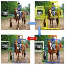
# 2.按照得分排序,取前12000个anchor,再nms,取前面2000个(在test的时候就变成了6000和300)
rois, roi_scores = self._proposal_layer(rpn_cls_prob, rpn_bbox_pred, "rois") # 256个anchors的类别(第一维)及位置(后四维)
# 获取属于rpn网络的label:通过对所有的anchor与所有的GT计算IOU,通过消除再图像外部的anchor,计算IOU>=0.7为正样本,IOU<0.3为负样本,
# 得到再理想情况下各自一半的256个正负样本(实际上正样本大多只有10-100个之间,相对负样本偏少)
rpn_labels = self._anchor_target_layer(rpn_cls_score, "anchor") #rpn_labels:特征图中每个位置对应的正样本、负样本还是不关注
# Try to have a deterministic order for the computing graph, for reproducibility
with tf.control_dependencies([rpn_labels]):
# 获得属于最后的分类网络的label
# 因为之前的anchor位置已经修正过了,所以这里又计算了一次经过proposal_layer修正后的box与GT的IOU来得到label
# 但是阈值不一样了,变成了大于等于0.5为1,小于为0,并且这里得到的正样本很少,通常只有2-20个,甚至有0个,
# 并且正样本最多为64个,负样本则有比较多个,相应的也重新计算了一次bbox_targets
# 另外,从RPN网络出来的2000余个rois中挑选256个
rois, _ = self._proposal_target_layer(rois, roi_scores, "rpn_rois") #通过post_nms_topN个anchors的位置及为1(正样本)的概率得到256个rois及对应信息
else:
if cfg.TEST.MODE == 'nms':
rois, _ = self._proposal_layer(rpn_cls_prob, rpn_bbox_pred, "rois")
elif cfg.TEST.MODE == 'top':
rois, _ = self._proposal_top_layer(rpn_cls_prob, rpn_bbox_pred, "rois")
else:
raise NotImplementedError
self._predictions["rpn_cls_score"] = rpn_cls_score # 每个位置的9个anchors是正样本还是负样本
self._predictions["rpn_cls_score_reshape"] = rpn_cls_score_reshape # 每个anchors是正样本还是负样本
self._predictions["rpn_cls_prob"] = rpn_cls_prob # 每个位置的9个anchors是正样本和负样本的概率
self._predictions["rpn_cls_pred"] = rpn_cls_pred # 每个位置的9个anchors预测的类别,[1,?,9,?]的列向量
self._predictions["rpn_bbox_pred"] = rpn_bbox_pred # 每个位置的9个anchors回归位置偏移
self._predictions["rois"] = rois # 256个anchors的类别(第一维)及位置(后四维)
return rois # 返回256个anchors的类别(第一维,训练时为每个anchors的类别,测试时全0)及位置(后四维)函数拆解:
先完成下图功能:

对应的代码:
    # vgg16提取后的特征图,先进行3*3卷积
    # 3*3的conv,作为rpn网络 cfg.RPN_CHANNELS=512是卷积后的通道数
    rpn = slim.conv2d(net_conv, cfg.RPN_CHANNELS, [3, 3], trainable=is_training, weights_initializer=initializer,
                        scope="rpn_conv/3x3")

    # 每个框进行2分类,判断前景还是背景
    # 1*1的conv,得到每个位置的9个anchors分类特征[1,?,?,9*2],
    rpn_cls_score = slim.conv2d(rpn, self._num_anchors * 2, [1, 1], trainable=is_training,
                                weights_initializer=initializer,
                                padding='VALID', activation_fn=None, scope='rpn_cls_score')
然后进行reshape,拿一张图片举个例子,图片的shape是(W,H,D=18),然后我们会把他reshape以进行softmax(进行softmax的matrix的一边需要等于num of class,在这里是一个二分类,即是否含有物体,所以是2)。所以我们会把(W,H,D)reshape成(2,9*W*H)。这里很重要!!!!对应的代码:
    # change it so that the score has 2 as its channel size
    # reshape成标准形式
    # [1,?,?,9*2]-->[1,?*9.?,2]  分类得分,每个点有9个anchors,每个anchors有2个得分
rpn_cls_score_reshape = self._reshape_layer(rpn_cls_score, 2, 'rpn_cls_score_reshape')然后我们进行softmax,得出对这9*W*H每一个的两个score,一个是有物体,一个是没有物体。对应的代码:
 # 每个anchors是正样本还是负样本。 以最后一维为特征长度,得到所有特征的概率[1,?*9.?,2]
    rpn_cls_prob_reshape = self._softmax_layer(rpn_cls_score_reshape, "rpn_cls_prob_reshape")
其他的语句:
    # 每个位置的9个anchors预测的类别。得到每个位置的9个anchors预测的类别,[1,?,9,?]的列向量
    rpn_cls_pred = tf.argmax(tf.reshape(rpn_cls_score_reshape, [-1, 2]), axis=1, name="rpn_cls_pred")

    # 变换回原始纬度,[1,?*9.?,2]-->[1,?,?,9*2]
    rpn_cls_prob = self._reshape_layer(rpn_cls_prob_reshape, self._num_anchors * 2, "rpn_cls_prob")

    # 1*1的conv,每个位置的9个anchors回归位置偏移[1,?,?,9*4]
    rpn_bbox_pred = slim.conv2d(rpn, self._num_anchors * 4, [1, 1], trainable=is_training,
                                weights_initializer=initializer,
                                padding='VALID', activation_fn=None, scope='rpn_bbox_pred')
最后一句完成下图的功能,rpn_bbox_pred对应下图红色圈出的部分:

以下至1.1.2主要是此部分代码 ,解析了以下4个函数。
完成从w*h*9个anchors中取2000个anchors,并第一次box regression操作。

1,_proposal_layer()
接下来调用_proposal_layer()函数,该函数主要是传入相关参数,并没有进行相关的数据操作,然后调用proposal_layer_tf()函数完成数据操作,最后返回rois, rpn_scores。
rois是筛选后的候选区域的个数(训练时为m=2000,测试时为m=300),rois为m*5维;
rpn_scores是rois为正样本的概率,rpn_scores为m*1维。
  '''
  _proposal_layer调用proposal_layer_tf,通过(w*h*9)*4个anchors,计算估计后的坐标
  (bbox_transform_inv_tf),并对坐标进行裁剪(clip_boxes_tf)及非极大值抑制
  (tf.image.non_max_suppression,可得到符合条件的索引indices)的anchors:rois
  及这些anchors为正样本的概率:rpn_scores。rois为m*5维,rpn_scores为m*1维,
  其中m为经过非极大值抑制后得到的候选区域个数(训练时2000个,测试时300个)。
  m*5的第一列为全为0的batch_inds,后4列为坐标(坐上+右下)
  '''
  # rpn_cls_prob  每个位置的9个anchors是正样本和负样本的概率
  # rpn_bbox_pred  每个位置的9个anchors回归位置偏移
  def _proposal_layer(self, rpn_cls_prob, rpn_bbox_pred, name):
    with tf.variable_scope(name) as scope:
      if cfg.USE_E2E_TF:
        #proposal_layer_tf()在lib/layer_utils/proposal_layer.py中定义
        rois, rpn_scores = proposal_layer_tf(
          rpn_cls_prob,      # rpn_cls_prob  每个位置的9个anchors是正样本和负样本的概率
          rpn_bbox_pred,     # rpn_bbox_pred  每个位置的9个anchors回归位置偏移
          self._im_info,     #图像信息
          self._mode,        # 'train'或者 'test'
          self._feat_stride, #原始图到特征图的缩放比例,此处为16
          self._anchors,     #此处传入生成的w*h*9个anchors
          self._num_anchors  #9
        )
      else:
        rois, rpn_scores = tf.py_func(proposal_layer,
                              [rpn_cls_prob,     #同上
                               rpn_bbox_pred,
                               self._im_info,
                               self._mode,
                               self._feat_stride,
                               self._anchors,
                               self._num_anchors],
                              [tf.float32, tf.float32], name="proposal")

      rois.set_shape([None, 5])
      rpn_scores.set_shape([None, 1])
return rois, rpn_scores1.1,proposal_layer_tf()
此函数主要功能是从w*h*9个anchors中筛选出2000个anchors及其为正样本的概率。 by:sxl --个人理解,如有错误,欢迎指正。该函数里面调用了bbox_transform_inv_tf()和clip_boxes_tf()完成相应功能,这两个函数会在下面解析。
'''
rpn_cls_prob,      # rpn_cls_prob  每个位置的9个anchors是正样本和负样本的概率 [1,?,?,18]
rpn_bbox_pred,     # rpn_bbox_pred  每个位置的9个anchors回归位置偏移 [1,?,?,36]
_im_info,          #图像信息
cfg_key(_mode),    # 'TRAIN'或者 'test'
_feat_stride,      #原始图到特征图的缩放比例,此处为16
_anchors,          #此处传入生成的w*h*9个anchors
_num_anchors       #9

此函数主要功能是从w*h*9个anchors中筛选出2000个anchors及其为正样本的概率。 by:sxl   --个人理解
'''
def proposal_layer_tf(rpn_cls_prob, rpn_bbox_pred, im_info, cfg_key, _feat_stride, anchors, num_anchors):
  if type(cfg_key) == bytes:
    cfg_key = cfg_key.decode('utf-8')
  pre_nms_topN = cfg[cfg_key].RPN_PRE_NMS_TOP_N    #12000
  post_nms_topN = cfg[cfg_key].RPN_POST_NMS_TOP_N  #训练时为2000,测试时为300
  nms_thresh = cfg[cfg_key].RPN_NMS_THRESH #nms的阈值,为0.7

  # Get the scores and bounding boxes  获取分数和边界框
  scores = rpn_cls_prob[:, :, :, num_anchors:] #[1,?,?,9]
  scores = tf.reshape(scores, shape=(-1,)) #[?,]
  rpn_bbox_pred = tf.reshape(rpn_bbox_pred, shape=(-1, 4)) #所有的anchors的四个坐标,[1,?,?,36]->[?,4]

  #bbox_transform_inv_tf()在lib/model/bbox_transform.py中定义  proposals[w*h*9,4]
  proposals = bbox_transform_inv_tf(anchors, rpn_bbox_pred) #已知anchors和偏移求预测的坐标 anchors[w*h*9,4]  rpn_bbox_pred[?,4]
  proposals = clip_boxes_tf(proposals, im_info[:2]) #限制预测坐标在原始图像上  proposals[w*h*9,4]

  # Non-maximal suppression
  # 通过nms得到分支最大的post_num_topN(训练时为2000,测试时为300)个坐标的索引 .执行完indices [?,]
  indices = tf.image.non_max_suppression(proposals, scores, max_output_size=post_nms_topN, iou_threshold=nms_thresh)

  boxes = tf.gather(proposals, indices) #根据索引得到post_nms_topN个对应的坐标  boxes [?,4]
  boxes = tf.to_float(boxes)  #将张量强制转换为float32类型。 boxes [?,4]
  scores = tf.gather(scores, indices) #得到post_nms_topN个对应的为1的概率,从'scores'中根据'indices'的参数值获取切片。
  scores = tf.reshape(scores, shape=(-1, 1)) #scores [?,]-》[?,1]

  # Only support single image as input  只支持单张图片的输入
  batch_inds = tf.zeros((tf.shape(indices)[0], 1), dtype=tf.float32) #按切片维度初始化一个全0列表
  blob = tf.concat([batch_inds, boxes], 1)  #post_nms_topN*1个batch_inds和post_nms_topN*4个坐标concat,得到post_nms_topN*5的blob

  return blob, scores
1.1.1,bbox_transform_inv_tf()
先了解一下边框回归,这里贴一下此篇文章的手抄版,为加深理解,自己手动抄了一个简化版(字太丑[手动捂脸])

'''
已知anchors和偏移求预测的坐标 boxes[w*h*9,4]  deltas[?,4]=deltas[w*h*9,4] 就是特征图有512维经过1*1降维到36维,然后reshape[?,4]
'''
def bbox_transform_inv_tf(boxes, deltas):
  boxes = tf.cast(boxes, deltas.dtype) #tf.cast()函数的作用是将boxes数据类型转换为deltas的数据类型
  widths = tf.subtract(boxes[:, 2], boxes[:, 0]) + 1.0 #宽
  heights = tf.subtract(boxes[:, 3], boxes[:, 1]) + 1.0 #高
  ctr_x = tf.add(boxes[:, 0], widths * 0.5) #中心x
  ctr_y = tf.add(boxes[:, 1], heights * 0.5) #中心x

  dx = deltas[:, 0] #预测的tx,初始值是特征图的值
  dy = deltas[:, 1] #预测的ty
  dw = deltas[:, 2] #预测的tw
  dh = deltas[:, 3] #预测的th

  # 平移变换
  pred_ctr_x = tf.add(tf.multiply(dx, widths), ctr_x) #自己抄的那张图里的公式1,已知xa,wa,tx反过来求预测的x中心坐标
  pred_ctr_y = tf.add(tf.multiply(dy, heights), ctr_y) #自己抄的那张图里的公式2,已知ya,ha,ty反过来求预测的y中心坐标

  #尺度缩放变换
  pred_w = tf.multiply(tf.exp(dw), widths)  #自己抄的那张图里的公式3,已知wa,tw反过来秋预测的w
  pred_h = tf.multiply(tf.exp(dh), heights) #自己抄的那张图里的公式4,已知ha,th反过来秋预测的h

  #目标输出,通过预测的中心点(pred_ctr_x,pred_ctr_y)和宽高pred_w及pred_h计算(x1,y1,x2,y2)
  pred_boxes0 = tf.subtract(pred_ctr_x, pred_w * 0.5) #预测框的起始和终点四个坐标
  pred_boxes1 = tf.subtract(pred_ctr_y, pred_h * 0.5)
  pred_boxes2 = tf.add(pred_ctr_x, pred_w * 0.5)
  pred_boxes3 = tf.add(pred_ctr_y, pred_h * 0.5)

  return tf.stack([pred_boxes0, pred_boxes1, pred_boxes2, pred_boxes3], axis=1)
1.1.2,clip_boxes_tf()
函数主要作用是:限制预测坐标在原始图像上,
tf.minimum(boxes[:, 0], im_info[1] - 1 保证预测的宽高不超出真实图片的宽高范围
tf.maximum(x,0) 保证预测宽高的值大于等于0
#限制预测坐标在原始图像上  proposals[w*h*9,4]
def clip_boxes_tf(boxes, im_info):
  '''
  tf.minimum(boxes[:, 0], im_info[1] - 1  保证预测的宽高不超出真实图片的宽高范围
  tf.maximum(x,0)  保证预测宽高的值大于等于0
  :param boxes:    预测边框信息
  :param im_info:  图像信息
  :return: 限制预测坐标在原始图像上的预测信息
  '''
  b0 = tf.maximum(tf.minimum(boxes[:, 0], im_info[1] - 1), 0)
  b1 = tf.maximum(tf.minimum(boxes[:, 1], im_info[0] - 1), 0)
  b2 = tf.maximum(tf.minimum(boxes[:, 2], im_info[1] - 1), 0)
  b3 = tf.maximum(tf.minimum(boxes[:, 3], im_info[0] - 1), 0)
  return tf.stack([b0, b1, b2, b3], axis=1)
下面重新开一篇文章解析下面这个模块


 376
376

 被折叠的 条评论
为什么被折叠?
被折叠的 条评论
为什么被折叠?
 到【灌水乐园】发言


