


 本文介绍了《Fundamentals of Statistical Signal Processing:Estimation Theory》一书的第2章内容,探讨了无偏估计量的概念,通过例子解释了无偏估计的性质。最小方差无偏估计(MVU)作为寻找最优估计的一种准则,但其存在性并不总是保证的。此外,文章还讨论了寻找MVU估计的挑战,并指出在矢量参数情况下MVU估计的定义和特性。
本文为《Steven M. Kay, Fundamentals of Statistical Signal Processing:Estimation Theory》一书的第2章。
1、无偏估计量
对未知参数进行估计,得到估计量。而所谓无偏估计,是指估计量的均值,等于未知参数的真值,即对未知参数
θ
\theta
θ,有
E
(
θ
^
)
=
θ
,
a
<
θ
<
b
,
(2.1)
\tag{2.1} {\rm E}( \hat \theta)=\theta,\quad a<\theta<b,
E(θ^)=θ,a<θ<b,(2.1)那么估计量是无偏的。
真值是确定的,估计量却是随机的,每次估计得到一个样本。因此无偏估计就是,估计量的均值等于真值。
【例2.1】AWGN中DC电平的无偏估计。
考虑观测
x
[
n
]
=
A
+
w
[
n
]
n
=
0
,
1
,
…
,
N
−
1
x[n]=A+w[n]\quad n=0,1,\ldots,N-1
x[n]=A+w[n]n=0,1,…,N−1其中
A
A
A是要估计的参数,
w
[
n
]
w[n]
w[n]是AWGN。参数
A
A
A可以取
−
∞
<
A
<
∞
-\infty<A<\infty
−∞<A<∞上的任何值。那么,
x
[
n
]
x[n]
x[n]的一个合理估计是
A
^
=
1
N
∑
n
=
0
N
−
1
x
[
n
]
,
(2.2)
\tag{2.2} \hat A=\frac{1}{N}\sum_{n=0}^{N-1}x[n],
A^=N1n=0∑N−1x[n],(2.2)即样本的均值。进一步,我们有
E
(
A
^
)
=
E
[
1
N
∑
n
=
0
N
−
1
x
[
n
]
]
=
1
N
∑
n
=
0
N
−
1
E
(
x
[
n
]
)
=
A
\begin{aligned} {\rm E}(\hat A)&={\rm E}\left[\frac{1}{N}\sum_{n=0}^{N-1}x[n]\right]\\ &=\frac{1}{N}\sum_{n=0}^{N-1}{\rm E}(x[n])\\ &=A \end{aligned}
E(A^)=E[N1n=0∑N−1x[n]]=N1n=0∑N−1E(x[n])=A因此,用样本均值作为估计量,是无偏的。
The restriction that
E
(
θ
^
)
=
θ
{\rm E}(\hat \theta)=\theta
E(θ^)=θ for all
θ
\theta
θ is an important one. Letting
θ
^
=
g
(
x
)
\hat \theta=g(\bf x)
θ^=g(x), where
x
=
[
x
[
0
]
,
x
[
1
]
,
…
,
x
[
N
−
1
]
]
T
{\bf x}=\left[ x[0],x[1],\ldots,x[N-1]\right]^T
x=[x[0],x[1],…,x[N−1]]T, it asserts that
E
(
θ
^
)
=
∫
g
(
x
)
p
(
x
;
θ
)
d
x
=
θ
f
o
r
a
l
l
θ
.
(2.3)
\tag{2.3} {\rm E}(\hat \theta)=\int g({\bf x})p({\bf x};\theta)d{\bf x}=\theta\quad {\rm for \ all\ \theta}.
E(θ^)=∫g(x)p(x;θ)dx=θfor all θ.(2.3)It is possible, however, that (2.3) may hold for some values of
θ
\theta
θ and not others, as the next example illustrate.
Example 2.2-Biased Estimator for DC Level in White Noise
Consider again Example 2.1 but with the modified sample mean estimator
A ˇ = 1 2 N ∑ n = 0 N − 1 x [ n ] . \check{A}=\frac{1}{2N}\sum_{n=0}^{N-1}x[n]. Aˇ=2N1n=0∑N−1x[n].Then
E ( A ˇ ) = 1 2 A { = A , i f A = 0 ≠ A , i f A ≠ 0. {\rm E}(\check{A})=\frac{1}{2}A\left\{\begin{aligned} =A,\ {\rm if}A=0\\ \ne A,\ {\rm if}A\ne 0. \end{aligned}\right. E(Aˇ)=21A{=A, ifA=0=A, ifA=0.It is seen that (2.3) holds for the modified estimator only for A = 0 A=0 A=0. Clearly, A ˇ \check{A} Aˇ is a biased estimator.
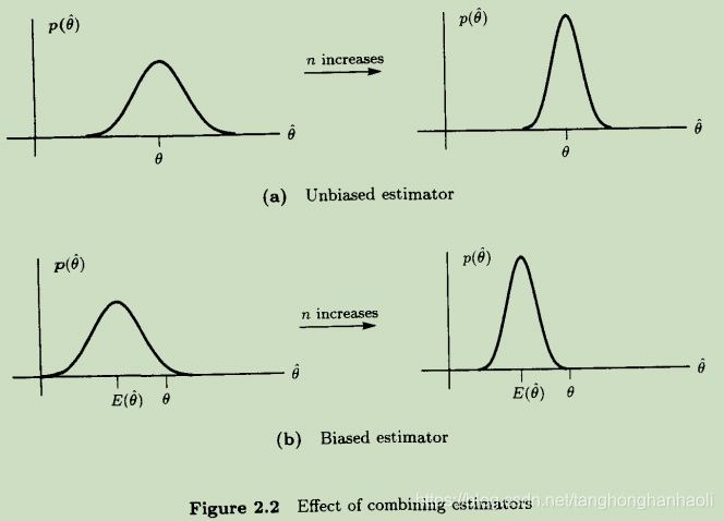
估计量是无偏的并不一定意味着它是一个好的估计量。这只能够保证,从平均上看能够得到真实值。另一方面,有偏估计量意味着存在系统误差,而系统误差是不应该出现的。持续的偏差总会使得估计结果很差。例如,当几个估计量被混合时,无偏特性具有重要意义(见习题2.4)。有时可能可以得到同一个参数的多种估计,例如
{
θ
^
1
,
θ
^
2
,
…
,
θ
^
n
}
\{\hat \theta_1,\hat \theta_2,\ldots,\hat \theta_n\}
{θ^1,θ^2,…,θ^n}。合理的步骤是把这些估计合并,希望能够通过对他们进行平均来得到更好的估计,即
θ
^
=
1
n
∑
i
=
1
n
θ
^
i
.
(2.4)
\tag{2.4} \hat \theta=\frac{1}{n}\sum_{i=1}^{n}\hat \theta_i.
θ^=n1i=1∑nθ^i.(2.4)假定所有的估计器都是无偏的,方差相等,彼此不相关,因此有
E
(
θ
^
)
=
θ
{\rm E}(\hat \theta)=\theta
E(θ^)=θ以及
v
a
r
(
θ
^
)
=
1
n
2
∑
i
=
1
n
v
a
r
(
θ
^
i
)
=
v
a
r
(
θ
^
1
)
n
\begin{aligned} {\rm var}(\hat \theta)&=\frac{1}{n^2}\sum_{i=1}^{n}{\rm var}(\hat \theta_i)\\ &=\frac{{\rm var}(\hat \theta_1)}{n} \end{aligned}
var(θ^)=n21i=1∑nvar(θ^i)=nvar(θ^1)因此求平均的统计量个数越多,则方差越小。最终,如果
n
→
∞
n\to \infty
n→∞,则
θ
^
→
θ
\hat \theta\to \theta
θ^→θ。 然而,如果估计器是有偏的,即
E
(
θ
^
)
=
θ
+
b
(
θ
)
{\rm E}(\hat \theta)=\theta+b(\theta)
E(θ^)=θ+b(θ),则
E
(
θ
^
)
=
1
n
∑
i
=
1
n
E
(
θ
^
i
)
=
θ
+
b
(
θ
)
.
\begin{aligned} {\rm E}(\hat \theta)&=\frac{1}{n}\sum_{i=1}^{n}{\rm E}(\hat \theta_i)\\ &=\theta+b(\theta). \end{aligned}
E(θ^)=n1i=1∑nE(θ^i)=θ+b(θ).因此,不论对多少个估计器进行平均,
θ
^
\hat \theta
θ^都不会收敛到真实值,如Figure 2.2所示。这里,通常将
b
(
θ
)
=
E
(
θ
^
)
−
θ
b(\theta)={\rm E}(\hat \theta)-\theta
b(θ)=E(θ^)−θ定义为估计器的偏差(bias)。
2、最小方差准则
在寻找最优估计时,我们需要采取一些最优化原则。很自然的,我们可以采用均方误差(mean square error,MSE),即
m
s
e
(
θ
^
)
=
E
[
(
θ
^
−
θ
)
2
]
.
(2.5)
\tag{2.5} {\rm mse}(\hat \theta)={\rm E}\left[(\hat \theta-\theta)^2\right].
mse(θ^)=E[(θ^−θ)2].(2.5)这个参数表述了估计量与真实值之间平方偏差的统计均值的大小。遗憾的是,采用这种自然准则的估计器是无法实现的,因为这个估计不能写成数据的函数。下面我们来看如何理解这个问题,我们将mse重写为
m
s
e
(
θ
^
)
=
E
{
[
(
θ
^
−
E
(
θ
^
)
+
(
E
(
θ
^
)
−
θ
)
]
2
}
=
v
a
r
(
θ
^
)
+
b
2
(
θ
)
(2.6)
\tag{2.6} \begin{aligned} {\rm mse}(\hat \theta)&={\rm E}\left\{\left[\left(\hat \theta-{\rm E}(\hat \theta \right)+\left({\rm E}(\hat \theta) -\theta\right) \right]^2\right\}\\ &={\rm var}(\hat \theta)+b^2(\theta) \end{aligned}
mse(θ^)=E{[(θ^−E(θ^)+(E(θ^)−θ)]2}=var(θ^)+b2(θ)(2.6)这意味着,MES的误差时由于估计量的方差,以及偏差所引起的。例如,对于Example 2.1,考虑修正的估计
A
ˇ
=
a
1
N
∑
n
=
0
N
−
1
x
[
n
]
\check A=a\frac{1}{N}\sum_{n=0}^{N-1}x[n]
Aˇ=aN1n=0∑N−1x[n]这里的
a
a
a为某常数。下面我们来确定使得MSE最小的
a
a
a值。由于
E
(
A
ˇ
)
=
a
A
{\rm E}(\check A)=aA
E(Aˇ)=aA,且
v
a
r
(
A
ˇ
)
=
a
2
σ
2
/
N
{\rm var}(\check A)=a^2\sigma^2/N
var(Aˇ)=a2σ2/N,我们从(2.6)可以得到
m
s
e
(
A
ˇ
)
=
a
2
σ
2
N
+
(
a
−
1
)
2
A
2
{\rm mse}(\check A)=\frac{a^2\sigma^2}{N}+(a-1)^2A^2
mse(Aˇ)=Na2σ2+(a−1)2A2对
a
a
a求微分,又
d
m
s
e
(
A
ˇ
)
d
a
=
2
a
σ
2
N
+
2
(
a
−
1
)
A
2
\frac{d{\rm mse}(\check A)}{da}=\frac{2a\sigma^2}{N}+2(a-1)A^2
dadmse(Aˇ)=N2aσ2+2(a−1)A2令其等于零,可以得到
a
a
a的最优值为
a
o
p
t
=
A
2
A
2
+
σ
2
/
N
a_{\rm opt}=\frac{A^2}{A^2+\sigma^2/N}
aopt=A2+σ2/NA2遗憾的是,从上面式子中可以看出,
a
a
a的最优值取决于未知参数
A
A
A,因此估计器是不可实现的。回想一下,之所以估计值与
A
A
A有关,是因为(2.6)中,偏差项与真实值有关。因此看起来,只要是与偏差有关的准则,都会导致估计器不可实现。尽管通常来说确实如此,偶尔也能找到可实现的最小MSE估计器[Bibby and Touterburg 1977, Rao 1973, Stoica and Moses 1990]。
从实际角度看,需要放弃最小MSE。另外一种方法是将偏差设为零,并找到最小化方差的估计,这种估计称为最小方差无偏估计(minimum variance unbiased, MUV)。从(2.6)可以看出,无偏差估计的MSE就是方差。
最小化无偏估计的方差,也能够使得估计误差
θ
^
−
θ
\hat \theta-\theta
θ^−θ的PDF更加集中在零点(问题2.7),因而出现大的估计误差的概率将变小。
3、最小方差无偏估计的存在性
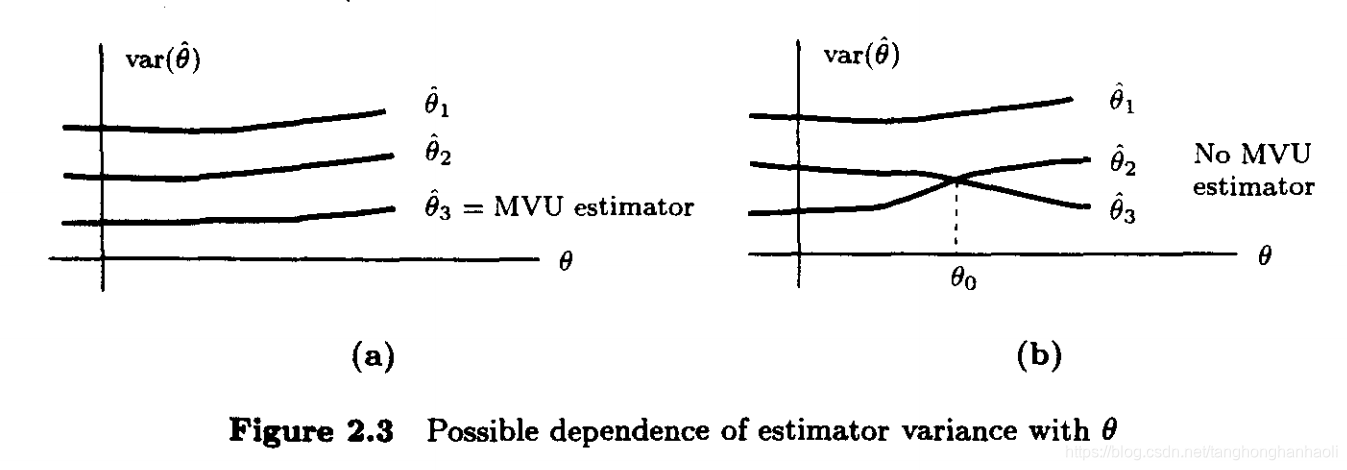
下面我们要讨论的问题是,MUV是否存在,或者说对于所有 θ \theta θ取值来说,是否都存在具有最小方差的无偏估计。图2.3中给出了两种可能情况。如果有三个无偏估计,其方差如图2.3a所示,显然 θ ^ 3 \hat \theta_3 θ^3为MVU估计。然而,对于2.3b中情况,没有MUV估计。这是由于若 θ ≤ θ 0 \theta \le \theta_0 θ≤θ0,则 θ ^ 2 \hat \theta_2 θ^2较好,而如果$ θ > θ 0 \theta > \theta_0 θ>θ0,则 θ ^ 3 \hat \theta_3 θ^3更好。在第一种情况中,为了强调对于所有 θ \theta θ的取值而言,方差都是最小的,有时将 θ ^ 3 \hat \theta_3 θ^3称为一致最小方差无偏估计。下面的例子将说明,通常来说,并非总存在MUV。
Example 2.3 不存在MUV估计的例子
如果PDF的形式随着 θ \theta θ而改变,那么可以预计最佳估计也随之改变。假定我们有两个独立的观测 x [ 0 ] x[0] x[0]和 x [ 1 ] x[1] x[1],其PDF为
x [ 0 ] ∼ N ( θ , 1 ) x [ 1 ] ∼ { N ( θ , 1 ) i f θ ≥ 0 N ( θ , 2 ) i f θ < 0 \begin{aligned} x[0]&\sim{\mathcal N}(\theta,1)\\ x[1]&\sim\left\{ \begin{aligned} {\mathcal N}(\theta,1)\ {\rm if}\ \theta\ge 0\\ {\mathcal N}(\theta,2)\ {\rm if}\ \theta< 0\\ \end{aligned}\right. \end{aligned} x[0]x[1]∼N(θ,1)∼{N(θ,1) if θ≥0N(θ,2) if θ<0 显然
θ ^ 1 = 1 2 ( x [ 0 ] + x [ 1 ] ) θ ^ 1 = 2 3 x [ 0 ] + 1 3 x [ 1 ] ) \hat \theta_1=\frac{1}{2}(x[0]+x[1])\\ \hat \theta_1=\frac{2}{3}x[0]+\frac{1}{3}x[1]) θ^1=21(x[0]+x[1])θ^1=32x[0]+31x[1])为无偏估计。为了计算方差,我们可以得到
v a r ( θ ^ 1 ) = 1 4 { v a r ( x [ 0 ] ) + v a r ( x [ 1 ] ) } v a r ( θ ^ 2 ) = 4 9 v a r ( x [ 0 ] ) + 1 9 v a r ( x [ 1 ] ) \begin{aligned} {\rm var}(\hat \theta_1)=\frac{1}{4}\left\{{\rm var}(x[0])+{\rm var}(x[1])\right\}\\ {\rm var}(\hat \theta_2)=\frac{4}{9}{\rm var}(x[0])+\frac{1}{9}{\rm var}(x[1]) \end{aligned} var(θ^1)=41{var(x[0])+var(x[1])}var(θ^2)=94var(x[0])+91var(x[1])因此有
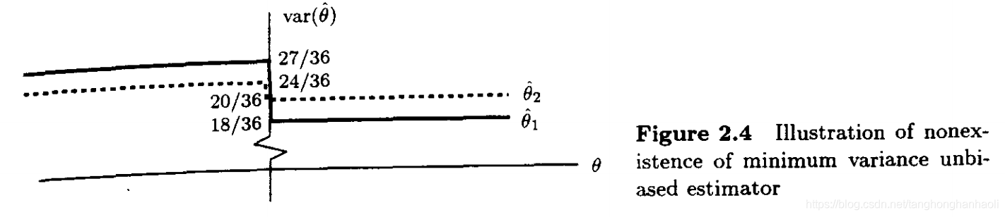
v a r ( θ ^ 1 ) = { 18 36 i f θ ≥ 0 27 36 i f θ < 0 {\rm var}(\hat \theta_1)=\left\{ \begin{aligned} \frac{18}{36}\quad {\rm if}\ \theta\ge 0\\ \frac{27}{36}\quad {\rm if}\ \theta< 0\\ \end{aligned}\right. var(θ^1)=⎩⎪⎨⎪⎧3618if θ≥03627if θ<0以及
v a r ( θ ^ 2 ) = { 20 36 i f θ ≥ 0 24 36 i f θ < 0 {\rm var}(\hat \theta_2)=\left\{ \begin{aligned} \frac{20}{36}\quad {\rm if }\ \theta\ge 0\\ \frac{24}{36}\quad {\rm if}\ \theta< 0\\ \end{aligned}\right. var(θ^2)=⎩⎪⎨⎪⎧3620if θ≥03624if θ<0方差如图2.4所示。显然,在这两种估计中,不存在MVU估计。
4、寻找最小方差无偏估计
即使存在MVU估计,我们也可能求不出来。没有一种“摇动曲柄”,总能求解出估计量的方法。在后面几章中,我们讨论几种可能的方法,包括:
- 确定Cramer-Rao下界(CRLB),并检视是否有某些估计能够满足(第3、4章)。
- 应用Rao-Blackwell-Lehmann-Scheffe(RBLS)定理(第5章)。
- 进一步将估计器的类型限定为不仅是无偏的,而且是线性的。随后对于所限定的类型,找到最小方差估计(第6章)。
方法1和2可能会得到MVU估计,而方法3只有估计量在数据中是线性时,才会得到MVU估计。
根据CRLB,我们知道对于任何无偏估计,方差一定大于或等于某个给定的值,如Figure 2.5所示。如果对于所有的 θ \theta θ值,存在方差等于CRLB的估计,则这个估计一定时MVU估计。这种情况下,根据CRLB理论可以立即得到估计。有可能不存在方差等于下界的估计,然而此时有可能仍然存在MVU估计,如Figure2.5中的 θ ^ 1 \hat \theta_1 θ^1所示。因此,我们必须使用Rao-Blackwell-Lehmann-Scheffe定理。这种方法首先找到一个有效使用所有数据的充分统计量,再找到作为 θ \theta θ无偏估计的这个充分量的一个函数。稍微对数据的PDF做些限定,这个方法可以保证得到无偏估计。第三种方法要求估计是线性的,这个限定有的时候是个严格的约束,并且选择最好的线性估计。当然,只有对于特殊的数据集,这个方法能够得到MVU估计。
5、扩展到矢量参数
如果
θ
=
[
θ
1
θ
2
…
θ
p
]
T
{\bm \theta}=[\theta_1\ \theta_2\ \ldots\ \theta_p]^{\rm T}
θ=[θ1 θ2 … θp]T为未知参数向量,如果对于
i
=
1
,
2
,
…
,
p
i=1,2,\ldots,p
i=1,2,…,p,有
E
(
θ
^
i
)
=
θ
i
,
a
i
<
θ
i
<
b
i
(2.7)
\tag{2.7} {\rm E}(\hat \theta_i)=\theta_i, \quad a_i<\theta_i<b_i
E(θ^i)=θi,ai<θi<bi(2.7)我们称估计
θ
^
=
[
θ
^
1
θ
^
2
…
θ
^
p
]
T
{\hat \bm \theta}=[\hat\theta_1\ \hat\theta_2\ \ldots\ \hat\theta_p]^{\rm T}
θ^=[θ^1 θ^2 … θ^p]T为无偏的。通过定义
E
(
θ
^
)
=
[
E
(
θ
^
1
)
E
(
θ
^
2
)
⋮
E
(
θ
^
p
)
]
{\rm E}({\hat \bm \theta})=\left[\begin{aligned} {\rm E}&(\hat \theta_1)\\ {\rm E}&(\hat \theta_2)\\ &\vdots\\ {\rm E}&(\hat \theta_p) \end{aligned}\right]
E(θ^)=⎣⎢⎢⎢⎢⎢⎡EEE(θ^1)(θ^2)⋮(θ^p)⎦⎥⎥⎥⎥⎥⎤我们可以等效地定义具有如下性质的无偏估计
E
(
θ
^
)
=
θ
{\rm E}(\hat \bm \theta)=\bm \theta
E(θ^)=θMVU估计具有附加性质,即
v
a
r
(
θ
^
i
)
{\rm var}(\hat \theta_i)
var(θ^i)在所有无偏估计中是最小的,这里
i
=
1
,
2
,
…
,
p
i=1,2,\ldots,p
i=1,2,…,p。


 741
741

 被折叠的 条评论
为什么被折叠?
被折叠的 条评论
为什么被折叠?
 到【灌水乐园】发言


