


参数估计:给定一个数据集,我们希望用一个给定的分布去拟合该数据集的分布,确定该分布的参数的过程就是参数估计。例如,我们用二项分布去拟合多次投掷硬币的情况,计算该二项分布的最优参数(出现正面的概率 θ \theta θ)就是参数估计。
下面,我们介绍在机器学习中常用的参数估计:极大似然估计 (Maximum Likelihood Estimation, MLE),最大后验概率估计 (Maximum A Posteriori, MAP)。在此之前,我们介绍一下参数估计中常用的一些概念.
-
频率学派 VS. 贝叶斯学派
- 频率学派:事件本身是服从某种参数 θ \theta θ固定的分布。频率学派认为概率即是频率,某次得到的样本 x \mathrm x x只是无数次可能的试验结果的一个具体实现,样本中未出现的结果不是不可能出现,只是这次抽样没有出现而已。在参数估计中,频率学派的代表是最大似然估计 MLE。
- 贝叶斯学派:参数 θ \theta θ也是随机分布的。贝叶斯学派认为只能依靠得到的样本 x \mathrm x x去做推断,而不能考虑那些有可能出现而未出现的结果。同时,贝叶斯学派引入了主观的概念,认为一个事件在发生之前,人们应该对它是有所认知,即先验概率 p ( θ ) p(\theta) p(θ),然后根据样本 x \mathrm x x 通过贝叶斯定理来得到后验概率 p ( θ ∣ x ) p(\theta\mid\mathrm x) p(θ∣x)。在参数估计中,贝叶斯学派的代表是最大后验概率估计 MAP。
-
概率 VS. 统计
概率与统计可以看成是互逆的概念。在http://stanford.edu/~lanhuong/refresher/notes/probstat-section3.pdf中对概念与统计推断作了简要概述:
• The basic problem of probability is: Given the distribution of the data, what are the properties (e.g. its expectation) of the outcomes (i.e. the data)?
• The basic problem of statistical inference is the inverse of probability: Given the outcomes, what can we say about the process that generated the data?
对于在机器学习中的常见问题,这里的data就是我们的训练样例,且机器学习的目的就是 say about the process that generated the data, 即学习生成训练样例的模型。
-
似然函数 VS. 概率函数
似然函数和概率函数的数学表达式一样,只是以不同的角度看待该函数表达式:- 若 θ \theta θ已知, x \mathrm x x是变量, P ( x ∣ θ ) P(\mathrm x\mid\theta) P(x∣θ) 被称为概率函数;
- 若 x \mathrm x x已知, θ \theta θ是变量, P ( x ∣ θ ) P(\mathrm x\mid\theta) P(x∣θ) 被称为似然函数;
一般为了保持符号的一致性,似然函数也经常写作 L ( θ ∣ x ) L(\theta\mid\mathrm x) L(θ∣x)。
极大似然估计 (MLE)
最大似然估计MLE的思想是,寻找使得观测到的数据出现概率最大的参数 θ \theta θ。
对于抛硬币来说,在一次抛硬币时,其结果的概率分布如下:
P
(
x
i
∣
θ
)
=
{
θ
,
x
i
=
1
1
−
θ
,
x
i
=
0
=
θ
x
i
(
1
−
θ
)
1
−
x
i
(1)
\begin{aligned} P(\mathrm x_i\mid\theta)&=\begin{cases} \theta,\quad\quad\hspace{4mm}\mathrm x_i=1\\ 1-\theta,\quad\mathrm x_i=0 \end{cases}\\ &=\theta^{\mathrm x_i}(1-\theta)^{1-\mathrm x_i} \end{aligned}\tag{1}
P(xi∣θ)={θ,xi=11−θ,xi=0=θxi(1−θ)1−xi(1)
其中
x
i
=
1
\mathrm x_i=1
xi=1表示第
i
i
i抛硬币时正面朝上。那么抛
N
N
N次硬币,其结果为
{
x
1
,
x
2
,
⋯
,
x
N
}
\{\mathrm x_1,\mathrm x_2,\cdots,\mathrm x_N\}
{x1,x2,⋯,xN}的概率为
P
(
x
1
,
x
2
,
⋯
,
x
N
∣
θ
)
=
∏
i
=
1
N
θ
x
i
(
1
−
θ
)
1
−
x
i
(2)
P(\mathrm x_1,\mathrm x_2,\cdots,\mathrm x_N\mid\theta)=\prod\limits_{i=1}^{N}\theta^{\mathrm x_i}(1-\theta)^{1-\mathrm x_i}\tag{2}
P(x1,x2,⋯,xN∣θ)=i=1∏Nθxi(1−θ)1−xi(2)
MLE就是寻找最优的
θ
\theta
θ最大化公式(2)的概率,即求解
θ
⋆
=
arg
max
θ
∏
i
=
1
N
θ
x
i
(
1
−
θ
)
1
−
x
i
(3)
\theta^\star=\arg\max_{\theta}\prod\limits_{i=1}^{N}\theta^{\mathrm x_i}(1-\theta)^{1-\mathrm x_i}\tag{3}
θ⋆=argθmaxi=1∏Nθxi(1−θ)1−xi(3)
对于优化问题(3),我们一般考虑将其转为对数目标函数,一方面可以将连乘转化为加和,防止计算溢出;另一方面使得目标函数更加精炼,便于通过求导求解最优解(连乘的导数不易计算)。为此,优化问题(3)可以转化为:
θ
⋆
=
arg
max
θ
∑
i
=
1
N
log
θ
x
i
(
1
−
θ
)
1
−
x
i
=
arg
max
θ
∑
i
=
1
N
x
i
log
θ
+
(
1
−
x
i
)
log
(
1
−
θ
)
(4)
\theta^\star=\arg\max_{\theta}\sum\limits_{i=1}^{N}\log{\theta^{\mathrm x_i}(1-\theta)^{1-\mathrm x_i}}=\arg\max_{\theta}\sum\limits_{i=1}^{N}\mathrm x_i\log{\theta}+(1-\mathrm x_i)\log{(1-\theta)}\tag{4}
θ⋆=argθmaxi=1∑Nlogθxi(1−θ)1−xi=argθmaxi=1∑Nxilogθ+(1−xi)log(1−θ)(4)
对(4)的目标函数对
θ
\theta
θ求导,并令导数为0 (目标函数为凹函数,在导数为0点取得极值),我们有:
∑
i
=
1
N
x
i
1
θ
+
(
1
−
x
i
)
−
1
1
−
θ
=
0
→
θ
=
∑
i
=
1
N
x
i
∑
i
=
1
N
1
(5)
\sum\limits_{i=1}^{N}\mathrm x_i\frac{1}{\theta}+(1-\mathrm x_i)\frac{-1}{1-\theta}=0\rightarrow\theta=\frac{\sum\nolimits_{i=1}^{N}\mathrm x_i}{\sum\nolimits_{i=1}^{N}1}\tag{5}
i=1∑Nxiθ1+(1−xi)1−θ−1=0→θ=∑i=1N1∑i=1Nxi(5)
公式(5)的结果比较符合直观:比如抛硬币10次,发现5次正面朝上,我们就说出现正面朝上的概率为0.5. 但是,也可能出现7次正面朝上的情况,这时我们说出现正面朝上的概率为0.7,显然这时与实际情况不符合(假定硬币是均匀的)。也就是说,当试验次数较少时,使用最大似然函数时的误差会较大。
上式(1)-(5)详细推导了离散的二项分布的最大似然估计(5)。对于常用的连续分布正态分布
N
(
μ
,
σ
2
)
\mathcal N(\mu,\sigma^2)
N(μ,σ2),我们只需要将公式(2)中的连乘项改为正态分布的概率密度函数,然后通过对数、求导为零,可以得到其最大似然估计为:
μ
=
1
N
∑
i
=
1
N
x
i
(6)
\mu=\frac{1}{N}\sum\limits_{i=1}^{N}x_i\tag{6}
μ=N1i=1∑Nxi(6)
σ 2 = 1 N ∑ i = 1 N ( x i − μ ) 2 (7) \sigma^2=\frac{1}{N}\sum\limits_{i=1}^{N}(x_i-\mu)^2\tag{7} σ2=N1i=1∑N(xi−μ)2(7)
其中,我们这里假设总共有 N N N个样本, x 1 , x 2 , ⋯ , x N x_1,x_2,\cdots,x_N x1,x2,⋯,xN。
最大后验概率估计 (MAP)
在最大后验概率MAP中,参数 θ \theta θ被看作为一个随机变量,服从某种概率分布,被称为先验概率 P ( θ ) P(\theta) P(θ)。
还是以上述抛硬币为例,考虑到先验概率,优化问题(3)被改写为:
θ
⋆
=
arg
max
θ
∏
i
=
1
N
θ
x
i
(
1
−
θ
)
1
−
x
i
p
(
θ
)
(8)
\theta^\star=\arg\max_{\theta}\prod\limits_{i=1}^{N}\theta^{\mathrm x_i}(1-\theta)^{1-\mathrm x_i}p(\theta)\tag{8}
θ⋆=argθmaxi=1∏Nθxi(1−θ)1−xip(θ)(8)
同样地,将公式(8)进行对数化可得:
θ
⋆
=
arg
max
θ
∑
i
=
1
N
log
θ
x
i
(
1
−
θ
)
1
−
x
i
p
(
θ
)
=
arg
max
θ
∑
i
=
1
N
x
i
log
θ
+
(
1
−
x
i
)
log
(
1
−
θ
)
+
log
p
(
θ
)
(9)
\begin{aligned} \theta^\star&=\arg\max_{\theta}\sum\limits_{i=1}^{N}\log{\theta^{\mathrm x_i}(1-\theta)^{1-\mathrm x_i}}p(\theta)\\&=\arg\max_{\theta}\sum\limits_{i=1}^{N}\mathrm x_i\log{\theta}+(1-\mathrm x_i)\log{(1-\theta)}+\log p(\theta)\tag{9} \end{aligned}
θ⋆=argθmaxi=1∑Nlogθxi(1−θ)1−xip(θ)=argθmaxi=1∑Nxilogθ+(1−xi)log(1−θ)+logp(θ)(9)
一般地,我们假设硬币是均匀地,即
p
(
θ
=
1
2
)
=
1
p(\theta=\frac{1}{2})=1
p(θ=21)=1,即此时参数
θ
\theta
θ时一个固定的未知量。此时,对(8)的目标函数对
θ
\theta
θ求导,并令导数为0,我们可以得到和公式(5)一样的结果。这说明,当先验分布为均匀分布时,MLE等价于MAP。但是,在最大后验概率中,我们可以假设
θ
\theta
θ是服从某一概率分布的。这里我们假设
θ
∼
N
(
μ
,
σ
)
\theta\sim N(\mu,\sigma)
θ∼N(μ,σ),即
p
(
θ
)
=
1
2
π
σ
e
−
(
θ
−
μ
)
2
2
σ
2
(10)
p(\theta)=\frac{1}{\sqrt{2\pi}\sigma}e^{-\frac{(\theta-\mu)^2}{2\sigma^2}}\tag{10}
p(θ)=2πσ1e−2σ2(θ−μ)2(10)
将公式(10)带入公式(9)可得:
θ
⋆
=
arg
max
θ
∑
i
=
1
N
x
i
log
θ
+
(
1
−
x
i
)
log
(
1
−
θ
)
+
log
1
2
π
σ
−
(
θ
−
μ
)
2
2
σ
2
(11)
\theta^\star=\arg\max_{\theta}\sum\limits_{i=1}^{N}\mathrm x_i\log{\theta}+(1-\mathrm x_i)\log{(1-\theta)}+\log{\frac{1}{\sqrt{2\pi}\sigma}}-\frac{(\theta-\mu)^2}{2\sigma^2}\tag{11}
θ⋆=argθmaxi=1∑Nxilogθ+(1−xi)log(1−θ)+log2πσ1−2σ2(θ−μ)2(11)
注意:由于正态分布的概率密度函数(10)是关于
θ
\theta
θ 的凹函数,公式(4)也是凹函数,所以公式(11)中的目标函数也是凹函数,所以我们可以利用导数为0取得最优的参数值
θ
⋆
\theta^\star
θ⋆。但是此时,我们一般无法得到如公式(5)一样简洁的解析表达式。在下面的具体实例中,我们直接给出目标函数的图像,从而可以形象地直接确定其最优解。对于比较复杂的目标函数,我们就需要借助其他迭代算法来求解了。
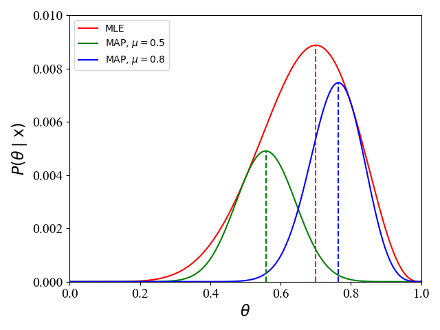
对于一个具体实例 (
μ
=
0.5
,
σ
=
0.1
\mu=0.5,\sigma=0.1
μ=0.5,σ=0.1,事件
x
\mathrm x
x为10次试验有7次为正面朝上),此时问题(8)中的目标函数为:
P
(
θ
∣
x
)
=
P
(
x
∣
θ
)
P
(
θ
)
=
θ
7
(
1
−
θ
)
3
10
2
π
e
−
50
(
θ
−
0.5
)
2
(10)
P(\theta\mid\mathrm x)=P(\mathrm x\mid\theta)P(\theta)=\theta^7(1-\theta)^3\frac{10}{\sqrt{2\pi}}e^{-50(\theta-0.5)^2}\tag{10}
P(θ∣x)=P(x∣θ)P(θ)=θ7(1−θ)32π10e−50(θ−0.5)2(10)
我们可以画出其函数曲线如下:
|
从图1中可以看出,当我们采用不同的先验概率分布时 ( μ = 0.5 , μ = 0.8 \mu=0.5,\mu=0.8 μ=0.5,μ=0.8),最终得到的参数也不同 ( θ ⋆ = 0.56 , θ ⋆ = 0.76 \theta^\star=0.56,\theta^\star=0.76 θ⋆=0.56,θ⋆=0.76)。在这里,我们假设硬币是均匀的,即正面朝上的概率为 θ = 0.5 \theta=0.5 θ=0.5,此时与MLE相比 ( θ = 0.7 \theta=0.7 θ=0.7),MAP的性能时好时坏,也就是说,MAP的性能与先验概率分布的选取有关。
等效情况
如前面所提及的,当先验概率为均匀分布时,MLE和MAP等效,因为此时 θ \theta θ服从均匀分布,没有提供有效的关于 θ \theta θ的先验信息。MLE和MAP等效的另一种情况就是:在频率学派所代表的MLE,当观测数据变大时(例子中对应抛硬币次数),这时观测数据的本身就提供了足够的信息,先验概率的影响变得微不足道,此时MLE和MAP等效,即最终估计的参数值 θ ⋆ \theta^\star θ⋆相同。如下图2和3,表示了当100次抛硬币70次为正面,和1000次抛硬币700次为正面时,对应的似然函数和后验概率函数:
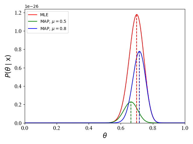 图2 图2
|
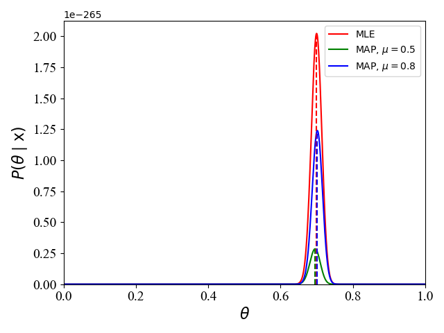 图3 图3
|
附录
下面给出图1-3的python源代码,由于代码简单,所以就没有注释
图1:
# -*- encoding: utf-8 -*-
"""
@File    : Parameter_Estimation_fig001.py
@Time    : 2020/5/31 14:46
@Author  : tengweitw
@Email   : tengweitw@foxmail.com
"""

import numpy as np
import matplotlib.pyplot as plt

# Set the format of labels
def LabelFormat(plt):
    ax = plt.gca()
    plt.tick_params(labelsize=14)
    labels = ax.get_xticklabels() + ax.get_yticklabels()
    [label.set_fontname('Times New Roman') for label in labels]
    font = {'family': 'Times New Roman',
            'weight': 'normal',
            'size': 16,
            }
    return font

sigma=0.1
mu1=0.5
mu2=0.8

theta=np.linspace(0,1,1000)
p_theta_x1=theta**7*(1-theta)**3/(np.sqrt(2*np.pi)*sigma)*np.exp(-np.square(theta-mu1)/2/np.square(sigma))
p_theta_x2=theta**7*(1-theta)**3/(np.sqrt(2*np.pi)*sigma)*np.exp(-np.square(theta-mu2)/2/np.square(sigma))

p_theta_x0=theta**7*(1-theta)**3/(np.sqrt(2*np.pi)*sigma)


p_max_ind0=np.argmax(p_theta_x0)
print(theta[p_max_ind0])

p_max_ind1=np.argmax(p_theta_x1)
print(theta[p_max_ind1])

p_max_ind2=np.argmax(p_theta_x2)
print(theta[p_max_ind2])


plt.figure()
plt.plot(theta,p_theta_x0,'r-')
plt.plot(theta,p_theta_x1,'g-')
plt.plot(theta,p_theta_x2,'b-')

plt.plot([theta[p_max_ind0],theta[p_max_ind0]],[0,p_theta_x0[p_max_ind0]],'r--')
plt.plot([theta[p_max_ind1],theta[p_max_ind1]],[0,p_theta_x1[p_max_ind1]],'g--')
plt.plot([theta[p_max_ind2],theta[p_max_ind2]],[0,p_theta_x2[p_max_ind2]],'b--')


plt.legend(["MLE",r"MAP, $\mu=0.5$",r"MAP, $\mu=0.8$"])

font = LabelFormat(plt)
plt.xlabel(r'$\theta$', font)
plt.ylabel(r'$P(\theta\mid\mathrm{x})$', font)
plt.xlim(0,1)
plt.ylim(0,0.01)
plt.show()
图2-3的源代码:
# -*- encoding: utf-8 -*-
"""
@File    : Parameter_Estimation_fig002.py
@Time    : 2020/5/31 16:01
@Author  : tengweitw
@Email   : tengweitw@foxmail.com
"""


import numpy as np
import matplotlib.pyplot as plt

# Set the format of labels
def LabelFormat(plt):
    ax = plt.gca()
    plt.tick_params(labelsize=14)
    labels = ax.get_xticklabels() + ax.get_yticklabels()
    [label.set_fontname('Times New Roman') for label in labels]
    font = {'family': 'Times New Roman',
            'weight': 'normal',
            'size': 16,
            }
    return font

sigma=0.1
mu1=0.5
mu2=0.8

theta=np.linspace(0,1,1000)
# Here to change 700 300 to 70 30 vice verse
p_theta_x1=theta**70*(1-theta)**30/(np.sqrt(2*np.pi)*sigma)*np.exp(-np.square(theta-mu1)/2/np.square(sigma))
p_theta_x2=theta**70*(1-theta)**30/(np.sqrt(2*np.pi)*sigma)*np.exp(-np.square(theta-mu2)/2/np.square(sigma))
p_theta_x0=theta**70*(1-theta)**30/(np.sqrt(2*np.pi)*sigma)


p_max_ind0=np.argmax(p_theta_x0)
print(theta[p_max_ind0])

p_max_ind1=np.argmax(p_theta_x1)
print(theta[p_max_ind1])

p_max_ind2=np.argmax(p_theta_x2)
print(theta[p_max_ind2])


plt.figure()
plt.plot(theta,p_theta_x0,'r-')
plt.plot(theta,p_theta_x1,'g-')
plt.plot(theta,p_theta_x2,'b-')

plt.plot([theta[p_max_ind0],theta[p_max_ind0]],[0,p_theta_x0[p_max_ind0]],'r--')
plt.plot([theta[p_max_ind1],theta[p_max_ind1]],[0,p_theta_x1[p_max_ind1]],'g--')
plt.plot([theta[p_max_ind2],theta[p_max_ind2]],[0,p_theta_x2[p_max_ind2]],'b--')


plt.legend(["MLE",r"MAP, $\mu=0.5$",r"MAP, $\mu=0.8$"])

font = LabelFormat(plt)
plt.xlabel(r'$\theta$', font)
plt.ylabel(r'$P(\theta\mid\mathrm{x})$', font)
plt.xlim(0,1)
plt.ylim(ymin=0)
plt.show()


 3383
3383

 被折叠的 条评论
为什么被折叠?
被折叠的 条评论
为什么被折叠?
 到【灌水乐园】发言


