


对比语言-图像预训练(Contrastive Language-Image Pre-Training),或称为 CLIP,是一种文本和图像编码工具,广泛用于许多流行的生成式 AI 模型中,例如 DALL-E 和 Stable Diffusion。
CLIP 本身并不是一个生成式 AI 模型,而是用于对齐文本编码和图像编码。如果存在图像的完美文字描述,CLIP 的目标就是为图像和文本创建相同的向量嵌入。这篇文章我们来学习如何使用 CLIP 编码(获取图像编码、获取文本编码、计算它们之间的余弦相似度),然后使用 CLIP 构建文本到图像的神经网络
1 编码
首先,我们加载本次练习所需的库。
# 导入 CSV 操作模块
import csv
# 导入用于文件匹配的模块
import glob
# 导入 NumPy 用于数值处理
import numpy as np
# 导入 PyTorch 主模块
import torch
# 导入 PyTorch 的函数式操作模块
import torch.nn.functional as F
# 导入 PyTorch 的优化器模块
from torch.optim import Adam
# 导入 torchvision 中的图像变换模块
import torchvision.transforms as transforms
# 导入 PyTorch 的数据集和数据加载模块
from torch.utils.data import Dataset, DataLoader

# 导入绘图工具 matplotlib
import matplotlib.pyplot as plt
# 导入 PIL 库处理图像
from PIL import Image
# 导入 torchvision 的图像保存和拼接函数
from torchvision.utils import save_image, make_grid
# 导入用于自动换行的模块
from textwrap import wrap

# 导入自己定义的.py文件
# 导入其他辅助工具
from utils import other_utils
# 导入 DDPM 模型相关工具
from utils import ddpm_utils
# 导入 UNet 相关工具
from utils import UNet_utils

# 设置设备为 CUDA(如可用)否则为 CPU
device = torch.device("cuda" if torch.cuda.is_available() else "cpu")
CLIP 有几个不同的变体,基于流行的图像识别神经网络:
# 导入 CLIP 库
import clip

# 显示可用的 CLIP 模型
clip.available_models()
输出如下:
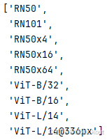
在本笔记本中,我们将使用 ViT-B/32,它是基于 Vision Transformer 架构构建的。它具有 512 个特征,我们稍后将把这些特征输入到我们的扩散模型中。
# 加载 CLIP 模型和预处理器
clip_model, clip_preprocess = clip.load("ViT-B/32")
# 设置模型为评估模式
clip_model.eval()
# 定义 CLIP 特征维度
CLIP_FEATURES = 512
1.1 图像编码
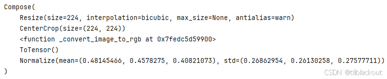
当我们加载 CLIP 时,它也会提供一组图像转换方法,我们可以使用这些方法将图像输入到 CLIP 模型中:
# 查看 CLIP 图像预处理操作
clip_preprocess
输出:
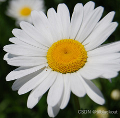
我们可以在一张花的照片上测试这一点。让我们从一朵如画的雏菊开始。
# 定义数据目录路径
DATA_DIR = "data/cropped_flowers/"
# 设置图像路径
img_path = DATA_DIR + "daisy/2877860110_a842f8b14a_m.jpg"
# 打开图像
img = Image.open(img_path)
# 显示图像
img.show()
输出:
我们可以通过首先使用 clip_preprocess 转换图像并将结果转换为张量来获取 CLIP 嵌入。由于 clip_model 期望的是一个图像批次,我们可以使用 np.stack 将处理后的图像变成一个包含一个元素的批次。
# 将图像转换为模型输入格式
clip_imgs = torch.tensor(np.stack([clip_preprocess(img)])).to(device)
# 打印图像张量的尺寸
clip_imgs.size()  # 输出torch.Size([1, 3, 224, 224])
然后,我们可以将这个批次传入 clip_model.encode_image 来把一张图片编码成一个语义特征向量。如果你想查看编码的具体内容,可以取消下面代码对 clip_img_encoding 的注释。当我们打印尺寸时,它显示了我们 1 张图像对应的 512 个特征。
# 获取图像编码
clip_img_encoding = clip_model.encode_image(clip_imgs)
# 打印编码的尺寸
print(clip_img_encoding.size())  # torch.Size([1, 512])
#clip_img_encoding
1.2 文本编码
现在我们已经有了图像编码,让我们看看是否可以得到一个匹配的文本编码。下面是一些不同的花的描述。和图像一样,文本在被 CLIP 编码之前也需要预处理。为此,CLIP 提供了一个 tokenize 函数,将每个词转换为整数。
# 定义文本描述列表
text_list = [
    "A round white daisy with a yellow center",
    "An orange sunflower with a big brown center",
    "A red rose bud"
]
# 将文本转换为 token
text_tokens = clip.tokenize(text_list).to(device)
# 打印 tokens
text_tokens
输出:
tensor([[49406,   320,  2522,  1579, 12865,   593,   320,  4481,  2119, 49407,
             0,     0,     0,     0,     0,     0,     0,     0,     0,     0,
             0,     0,     0,     0,     0,     0,     0,     0,     0,     0,
             0,     0,     0,     0,     0,     0,     0,     0,     0,     0,
             0,     0,     0,     0,     0,     0,     0,     0,     0,     0,
             0,     0,     0,     0,     0,     0,     0,     0,     0,     0,
             0,     0,     0,     0,     0,     0,     0,     0,     0,     0,
             0,     0,     0,     0,     0,     0,     0],
        [49406,   550,  4287, 21559,   593,   320,  1205,  2866,  2119, 49407,
             0,     0,     0,     0,     0,     0,     0,     0,     0,     0,
             0,     0,     0,     0,     0,     0,     0,     0,     0,     0,
             0,     0,     0,     0,     0,     0,     0,     0,     0,     0,
             0,     0,     0,     0,     0,     0,     0,     0,     0,     0,
             0,     0,     0,     0,     0,     0,     0,     0,     0,     0,
             0,     0,     0,     0,     0,     0,     0,     0,     0,     0,
             0,     0,     0,     0,     0,     0,     0],
        [49406,   320,   736,  3568, 10737, 49407,     0,     0,     0,     0,
             0,     0,     0,     0,     0,     0,     0,     0,     0,     0,
             0,     0,     0,     0,     0,     0,     0,     0,     0,     0,
             0,     0,     0,     0,     0,     0,     0,     0,     0,     0,
             0,     0,     0,     0,     0,     0,     0,     0,     0,     0,
             0,     0,     0,     0,     0,     0,     0,     0,     0,     0,
             0,     0,     0,     0,     0,     0,     0,     0,     0,     0,
             0,     0,     0,     0,     0,     0,     0]], device='cuda:0',
       dtype=torch.int32)
然后,我们可以将这些 token 输入 encode_text 以获得文本编码。如果你想查看编码结果,可以取消对 clip_text_encodings 的注释。和图像编码类似,每个文本条目会返回 512 个特征。
# 获取文本编码
clip_text_encodings = clip_model.encode_text(text_tokens).float()
# 打印编码的尺寸
print(clip_text_encodings.size())
#clip_text_encodings
1.3 相似度(Similarity)
为了看看哪一段文本描述最符合这张雏菊图片,我们可以计算文本编码与图像编码之间的 余弦相似度(cosine similarity)。当余弦相似度为 1 时,说明是完美匹配;当相似度为 -1 时,说明两个编码是完全相反的。
余弦相似度等价于一个 点积(dot product),并且每个向量都被它们的模长归一化。换句话说,每个向量的模长变成了 1。我们可以使用以下公式计算点积:
X
⋅
Y
=
∑
i
=
1
n
x
i
y
i
=
x
1
y
1
+
x
2
y
2
+
⋯
+
x
n
y
n
X \cdot Y = \sum_{i=1}^{n} x_i y_i = x_1y_1 + x_2 y_2 + \cdots + x_n y_n
X⋅Y=i=1∑nxiyi=x1y1+x2y2+⋯+xnyn
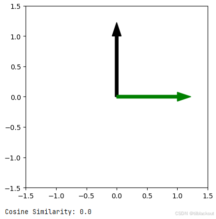
我们来练习一下。试着把 x1、y1、x2 和 y2 改成 -1 到 1 之间的值。当箭头方向一致时,余弦相似度为 1;当箭头方向相反时,余弦相似度为 -1。
一些建议的数值组合:
x1, y1 = [0, 0.5],x2, y2 = [0, 1]x1, y1 = [0, -1],x2, y2 = [0, 0.5]x1, y1 = [1, 1],x2, y2 = [0, 1]
# 设置第一个箭头的坐标
x1, y1 = [0, 1] # 修改这里
# 设置第二个箭头的坐标
x2, y2 = [1, 0] # 修改这里

# 构建向量
p1 = [x1, y1]
p2 = [x2, y2]

# 设置箭头宽度
arrow_width = 0.05
# 设置图像为正方形坐标系
plt.axis('square')
plt.xlim(-1.5, 1.5)
plt.ylim(-1.5, 1.5)
# 画出第一个箭头(黑色)
plt.arrow(0, 0, x1, y1, width=arrow_width, color="black")
# 画出第二个箭头(绿色)
plt.arrow(0, 0, x2, y2, width=arrow_width, color="green")
# 显示图像
plt.show()

# 计算余弦相似度
cosine = np.dot(p1, p2) / (np.linalg.norm(p1) * np.linalg.norm(p2))
print("Cosine Similarity:", cosine)
输出如下:
余弦相似度也可以应用于多维向量,尽管在二维图上难以可视化。试着修改下面的数值。如果 p1 是 p2 的倍数会发生什么?
# 设置两个向量
p1 = [1, 8, 6, 7]
p2 = [5, 3, 0, 9]

# 计算多维向量的余弦相似度
cosine = np.dot(p1, p2) / (np.linalg.norm(p1) * np.linalg.norm(p2))
print("Cosine Similarity:", cosine) # 输出: 0.7004760286167305
我们来试试计算我们 CLIP 编码的相似度得分。
# 对图像编码进行归一化
clip_img_encoding /= clip_img_encoding.norm(dim=-1, keepdim=True)
# 对文本编码进行归一化
clip_text_encodings /= clip_text_encodings.norm(dim=-1, keepdim=True)
# 计算余弦相似度
similarity = (clip_text_encodings * clip_img_encoding).sum(-1)
下面输出三个文本分别与图片的余弦相似度:
# 遍历输出每段文本及其对应相似度
for idx, text in enumerate(text_list):
    print(text, " - ", similarity[idx])
输出:
A round white daisy with a yellow center  -  tensor(0.3704, device='cuda:0', grad_fn=<SelectBackward0>)
An orange sunflower with a big brown center  -  tensor(0.2471, device='cuda:0', grad_fn=<SelectBackward0>)
A red rose bud  -  tensor(0.1767, device='cuda:0', grad_fn=<SelectBackward0>)
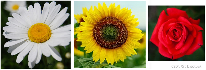
我们再多练习一下。下面我们加入了一张向日葵和一张玫瑰的图片。
# 设置三张图片的路径
img_paths = [
    DATA_DIR + "daisy/2877860110_a842f8b14a_m.jpg",
    DATA_DIR + "sunflowers/2721638730_34a9b7a78b.jpg",
    DATA_DIR + "roses/8032328803_30afac8b07_m.jpg"
]

# 读取图像
imgs = [Image.open(path) for path in img_paths]
# 显示图像
for img in imgs:
    img.show()
输出如下:
下面是 get_img_encodings 函数,用于从 PIL 图像生成 CLIP 编码。
# 定义图像编码函数
def get_img_encodings(imgs):
    # 对图像进行预处理
    processed_imgs = [clip_preprocess(img) for img in imgs]
    # 转换为张量并转移到设备上
    clip_imgs = torch.tensor(np.stack(processed_imgs)).to(device)
    # 编码图像
    clip_img_encodings = clip_model.encode_image(clip_imgs)
    return clip_img_encodings
# 获取图像编码
clip_img_encodings = get_img_encodings(imgs)
clip_img_encodings
输出如下:
tensor([[-0.2722, -0.0156, -0.1793,  ...,  0.5815,  0.0871, -0.1442],
        [ 0.2590, -0.1023, -0.3442,  ..., -0.0083,  0.4956,  0.0825],
        [-0.0613,  0.4138,  0.0088,  ...,  0.3269,  0.4639, -0.1385]],
       device='cuda:0', dtype=torch.float16, grad_fn=<MmBackward0>)
现在我们可以反复测试,写出能很好描述上述图像的文本,然后看一下是否能得到较高的相似度得分。
# 设置文本列表
text_list = [
    "A round white daisy with a yellow center",
    "An orange sunflower with a big brown center",
    "A deep red rose flower"
]
# 文本转 token 并编码
text_tokens = clip.tokenize(text_list).to(device)
clip_text_encodings = clip_model.encode_text(text_tokens).float()
clip_text_encodings
输出:
tensor([[-0.2874, -0.1919,  0.1517,  ..., -0.2301,  0.0572, -0.1427],
        [ 0.0701,  0.0188,  0.2164,  ..., -0.2563, -0.1208,  0.1393],
        [-0.2050,  0.2688,  0.2397,  ..., -0.5176, -0.0798, -0.2930]],
       device='cuda:0', grad_fn=<ToCopyBackward0>)
我们想比较每一个文本和图像的组合。为此,我们可以对每个文本编码进行 repeat,对每个图像编码进行 repeat_interleave。
# 对编码归一化
clip_img_encodings /= clip_img_encodings.norm(dim=-1, keepdim=True)
clip_text_encodings /= clip_text_encodings.norm(dim=-1, keepdim=True)
# 获取图像和文本数量
n_imgs = len(imgs)
n_text = len(text_list)
# 重复文本编码 n_imgs 次
repeated_clip_text_encodings = clip_text_encodings.repeat(n_imgs, 1)
# 对图像编码进行交错重复 n_text 次
repeated_clip_img_encoding = clip_img_encodings.repeat_interleave(n_text, dim=0)
# 计算所有组合的相似度
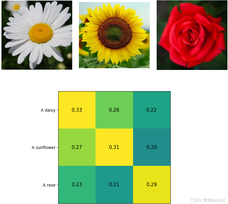
similarity = (repeated_clip_text_encodings * repeated_clip_img_encoding).sum(-1)
# 重塑为矩阵:每行是图像,每列是文本
similarity = torch.unflatten(similarity, 0, (n_text, n_imgs))
similarity
输出:
tensor([[0.3257, 0.2693, 0.2328],
        [0.2559, 0.3112, 0.2081],
        [0.2162, 0.1985, 0.2937]], device='cuda:0', grad_fn=<ViewBackward0>)
我们来可视化比较一下。理想情况下,从左上角到右下角的对角线应该是亮黄色(表示相似度高),其余的应该是蓝色(相似度低)。
# 设置图像显示区域
fig = plt.figure(figsize=(10, 10))
gs = fig.add_gridspec(2, 3, wspace=.1, hspace=0)

# 显示图像在上面一行
for i, img in enumerate(imgs):
    ax = fig.add_subplot(gs[0, i])
    ax.axis("off")
    plt.imshow(img)

# 显示相似度矩阵在下方
ax = fig.add_subplot(gs[1, :])
plt.imshow(similarity.detach().cpu().numpy().T, vmin=0.1, vmax=0.3)

# 设置标签格式
labels = [ '\n'.join(wrap(text, 20)) for text in text_list ]
plt.yticks(range(n_text), labels, fontsize=10)
plt.xticks([])

# 显示数值在格子中间
for x in range(similarity.shape[1]):
    for y in range(similarity.shape[0]):
        plt.text(x, y, f"{similarity[x, y]:.2f}", ha="center", va="center", size=12)
输出如下:
2 CLIP 数据集
刚刚我们使用花的种类作为标签。这一次,我们将使用 CLIP 编码作为标签。
如果 CLIP 的目标是将文本编码与图像编码对齐,那么我们是否需要为数据集中的每张图片提供文本描述?我们的假设是:我们并不需要文本描述,只需要图像的 CLIP 编码就可以建立一个文本生成图像的模型。
为了验证这个假设,我们将 CLIP 编码作为“标签”添加到数据集中。虽然在每个批次的数据增强图像上实时运行 CLIP 会更准确,但也会更慢。我们可以通过预处理并提前存储编码来加快速度。
我们可以使用 glob 来列出所有图像文件的路径:
# 获取数据集中所有 JPG 图像路径
data_paths = glob.glob(DATA_DIR + '*/*.jpg', recursive=True)
# 打印前五个路径
data_paths[:5]
输出如下:
['data/cropped_flowers/sunflowers/3062794421_295f8c2c4e.jpg',
 'data/cropped_flowers/sunflowers/5076821914_c21b58fd4c_m.jpg',
 'data/cropped_flowers/sunflowers/5994569021_749d5e2da3_n.jpg',
 'data/cropped_flowers/sunflowers/24459750_eb49f6e4cb_m.jpg',
 'data/cropped_flowers/sunflowers/4814106562_7c3564d2d9_n.jpg']
下面这段代码会对每个文件路径执行以下操作:
- 打开该路径对应的图像,存储为
img - 对图像进行预处理,获取 CLIP 编码,存储为
clip_img - 将 CLIP 编码从张量转换为 Python 列表
- 将文件路径和 CLIP 编码作为一行写入 CSV 文件中
# 定义保存编码的 CSV 文件路径
csv_path = 'clip.csv'

# 打开 CSV 文件进行写入
with open(csv_path, 'w', newline='') as csvfile:
    writer = csv.writer(csvfile, delimiter=',')
    for idx, path in enumerate(data_paths):
        img = Image.open(path)
        clip_img = torch.tensor(np.stack([clip_preprocess(img)])).to(device)
        label = clip_model.encode_image(clip_img)[0].tolist()
        writer.writerow([path] + label)
我们可以继续使用前面写的的图像转换方式:
# 设置图像尺寸和通道数
IMG_SIZE = 32  # 由于 stride 和 pooling,尺寸必须是 2 的倍数
IMG_CH = 3
BATCH_SIZE = 128
INPUT_SIZE = (IMG_CH, IMG_SIZE, IMG_SIZE)

# 定义预处理转换
pre_transforms = [
    transforms.Resize(IMG_SIZE),
    transforms.ToTensor(),  # 数据缩放到 [0,1]
    transforms.Lambda(lambda t: (t * 2) - 1)  # 缩放到 [-1,1]
]
pre_transforms = transforms.Compose(pre_transforms)

# 定义数据增强的随机变换
random_transforms = [
    transforms.RandomCrop(IMG_SIZE),
    transforms.RandomHorizontalFlip(),
]
random_transforms = transforms.Compose(random_transforms)
下面是初始化我们新数据集的代码。我们设置了一个变量 preprocessed_clip,表示我已经把图像的 CLIP 编码提前算好并写进了 CSV 文件,每次加载直接用,如果为真则会在 __init__ 中预加载到 GPU 上。如果为假,则在训练时实时计算 CLIP 编码,它能得到稍微好一点的结果,但运行速度会慢很多。
# 定义自定义数据集
class MyDataset(Dataset):
    def __init__(self, csv_path, preprocessed_clip=True):
        self.imgs = []
        self.preprocessed_clip = preprocessed_clip
        if preprocessed_clip:
            self.labels = torch.empty(
                len(data_paths), CLIP_FEATURES, dtype=torch.float, device=device
            )

        with open(csv_path, newline='') as csvfile:
            reader = csv.reader(csvfile, delimiter=',')
            for idx, row in enumerate(reader):
                img = Image.open(row[0])
                self.imgs.append(pre_transforms(img).to(device))
                if preprocessed_clip:
                    label = [float(x) for x in row[1:]]
                    self.labels[idx, :] = torch.FloatTensor(label).to(device)

    def __getitem__(self, idx):
        img = random_transforms(self.imgs[idx])
        if self.preprocessed_clip:
            label = self.labels[idx]
        else:
            batch_img = img[None, :, :, :]
            encoded_imgs = clip_model.encode_image(clip_preprocess(batch_img))
            label = encoded_imgs.to(device).float()[0]
        return img, label

    def __len__(self):
        return len(self.imgs)
# 加载数据集并创建数据加载器
train_data = MyDataset(csv_path)
dataloader = DataLoader(train_data, batch_size=BATCH_SIZE, shuffle=True, drop_last=True)
UNet 模型与上一次相同,不过有一个小改变。我们不再使用类别数量作为 c_embed_dim,而是使用 CLIP_FEATURES。之前的 c 是指类别(class),这次则是上下文(context)。
# 定义时间步数与 beta 计划
T = 400
B_start = 0.0001
B_end = 0.02
B = torch.linspace(B_start, B_end, T).to(device)

# 初始化 DDPM 和 UNet 模型
ddpm = ddpm_utils.DDPM(B, device)
model = UNet_utils.UNet(
    T, IMG_CH, IMG_SIZE, down_chs=(256, 256, 512), t_embed_dim=8, c_embed_dim=CLIP_FEATURES
)
# 打印参数数量
print("Num params: ", sum(p.numel() for p in model.parameters()))  # 输出44900355
# 使用 torch.compile 加速训练
model_flowers = torch.compile(model.to(device))
get_context_mask 函数也需要一点改动。因为我们不再使用 one-hot 编码标签,而是用 CLIP 编码。我们仍然会随机将编码中的值置 0,以帮助模型学习没有上下文的情况。
# 生成上下文掩码,随机置 0
def get_context_mask(c, drop_prob):
    c_mask = torch.bernoulli(torch.ones_like(c).float() - drop_prob).to(device)
    return c_mask
sample_w 函数基本没变,它被移到了 ddpm_utils.py 的底部,以下是ddpm_utils.py的内容:
import torch
import torch.nn.functional as F
import matplotlib.pyplot as plt

from utils import other_utils


class DDPM:
    def __init__(self, B, device):
        self.B = B
        self.T = len(B)
        self.device = device

        # Forward diffusion variables
        self.a = 1.0 - self.B
        self.a_bar = torch.cumprod(self.a, dim=0)
        self.sqrt_a_bar = torch.sqrt(self.a_bar)  # Mean Coefficient
        self.sqrt_one_minus_a_bar = torch.sqrt(1 - self.a_bar)  # St. Dev. Coefficient

        # Reverse diffusion variables
        self.sqrt_a_inv = torch.sqrt(1 / self.a)
        self.pred_noise_coeff = (1 - self.a) / torch.sqrt(1 - self.a_bar)

    def q(self, x_0, t):
        """
        The forward diffusion process
        Returns the noise applied to an image at timestep t
        x_0: the original image
        t: timestep
        """
        t = t.int()
        noise = torch.randn_like(x_0)
        sqrt_a_bar_t = self.sqrt_a_bar[t, None, None, None]
        sqrt_one_minus_a_bar_t = self.sqrt_one_minus_a_bar[t, None, None, None]

        x_t = sqrt_a_bar_t * x_0 + sqrt_one_minus_a_bar_t * noise
        return x_t, noise

    def get_loss(self, model, x_0, t, *model_args):
        x_noisy, noise = self.q(x_0, t)
        noise_pred = model(x_noisy, t, *model_args)
        return F.mse_loss(noise, noise_pred)

    @torch.no_grad()
    def reverse_q(self, x_t, t, e_t):
        """
        The reverse diffusion process
        Returns the an image with the noise from time t removed and time t-1 added.
        model: the model used to remove the noise
        x_t: the noisy image at time t
        t: timestep
        model_args: additional arguments to pass to the model
        """
        t = t.int()
        pred_noise_coeff_t = self.pred_noise_coeff[t]
        sqrt_a_inv_t = self.sqrt_a_inv[t]
        u_t = sqrt_a_inv_t * (x_t - pred_noise_coeff_t * e_t)
        if t[0] == 0:  # All t values should be the same
            return u_t  # Reverse diffusion complete!
        else:
            B_t = self.B[t - 1]  # Apply noise from the previos timestep
            new_noise = torch.randn_like(x_t)
            return u_t + torch.sqrt(B_t) * new_noise

    @torch.no_grad()
    def sample_images(self, model, img_ch, img_size, ncols, *model_args, axis_on=False):
        # Noise to generate images from
        x_t = torch.randn((1, img_ch, img_size, img_size), device=self.device)
        plt.figure(figsize=(8, 8))
        hidden_rows = self.T / ncols
        plot_number = 1

        # Go from T to 0 removing and adding noise until t = 0
        for i in range(0, self.T)[::-1]:
            t = torch.full((1,), i, device=self.device).float()
            e_t = model(x_t, t, *model_args)  # Predicted noise
            x_t = self.reverse_q(x_t, t, e_t)
            if i % hidden_rows == 0:
                ax = plt.subplot(1, ncols+1, plot_number)
                if not axis_on:
                    ax.axis('off')
                other_utils.show_tensor_image(x_t.detach().cpu())
                plot_number += 1
        plt.show()


# For use in Clip
@torch.no_grad()
def sample_w(
    model, ddpm, input_size, T, c, device, w_tests=None, store_freq=10
):
    if w_tests is None:
        w_tests = [-2.0, -1.0, -0.5, 0.0, 0.5, 1.0, 2.0]
    # Preprase "grid of samples" with w for rows and c for columns
    n_samples = len(w_tests) * len(c)

    # One w for each c
    w = torch.tensor(w_tests).float().repeat_interleave(len(c))
    w = w[:, None, None, None].to(device)  # Make w broadcastable
    x_t = torch.randn(n_samples, *input_size).to(device)

    # One c for each w
    c = c.repeat(len(w_tests), 1)

    # Double the batch
    c = c.repeat(2, 1)

    # Don't drop context at test time
    c_mask = torch.ones_like(c).to(device)
    c_mask[n_samples:] = 0.0

    x_t_store = []
    for i in range(0, T)[::-1]:
        # Duplicate t for each sample
        t = torch.tensor([i]).to(device)
        t = t.repeat(n_samples, 1, 1, 1)

        # Double the batch
        x_t = x_t.repeat(2, 1, 1, 1)
        t = t.repeat(2, 1, 1, 1)

        # Find weighted noise
        e_t = model(x_t, t, c, c_mask)
        e_t_keep_c = e_t[:n_samples]
        e_t_drop_c = e_t[n_samples:]
        e_t = (1 + w) * e_t_keep_c - w * e_t_drop_c

        # Deduplicate batch for reverse diffusion
        x_t = x_t[:n_samples]
        t = t[:n_samples]
        x_t = ddpm.reverse_q(x_t, t, e_t)

        # Store values for animation
        if i % store_freq == 0 or i == T or i < 10:
            x_t_store.append(x_t)

    x_t_store = torch.stack(x_t_store)
    return x_t, x_t_store
我们还要重新创建 sample_flowers 函数。这次它接收一个 text_list,并将其转换为 CLIP 编码。
# 采样函数,根据文本描述生成图像
def sample_flowers(text_list):
    text_tokens = clip.tokenize(text_list).to(device)
    c = clip_model.encode_text(text_tokens).float()
    x_gen, x_gen_store = ddpm_utils.sample_w(model, ddpm, INPUT_SIZE, T, c, device)
    return x_gen, x_gen_store
现在我们训练模型,大约训练 50 个 epochs 后,模型就能生成一些可识别的图像;训练 100 个 epochs 时,就能达到较好效果。
# 设置训练超参数
epochs=100
c_drop_prob = 0.1
lrate = 1e-4
save_dir = "05_images/"
# 初始化优化器
optimizer = torch.optim.Adam(model.parameters(), lr=lrate)

# 模型进入训练模式
model.train()
for epoch in range(epochs):
    for step, batch in enumerate(dataloader):
        optimizer.zero_grad()
        t = torch.randint(0, T, (BATCH_SIZE,), device=device).float()
        x, c = batch
        c_mask = get_context_mask(c, c_drop_prob)
        loss = ddpm.get_loss(model_flowers, x, t, c, c_mask)
        loss.backward()
        optimizer.step()

    print(f"Epoch {epoch} | Step {step:03d} | Loss: {loss.item()}")
    if epoch % 5 == 0 or epoch == int(epochs - 1):
        x_gen, x_gen_store = sample_flowers(text_list)
        grid = make_grid(x_gen.cpu(), nrow=len(text_list))
        save_image(grid, save_dir + f"image_ep{epoch:02}.png")
        print("saved images in " + save_dir + f" for episode {epoch}")
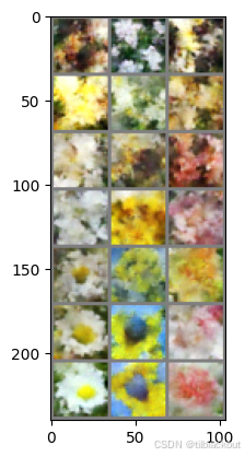
现在模型训练好了,让我们试试看给它一些数据集中没有的提示词会发生什么?将提示词精心设计以获得你想要结果的过程被称为 提示词工程(prompt engineering),如你所见,这非常依赖于模型训练时的数据类型。
# 修改这里的提示词
text_list = [
    "A daisy",
    "A sunflower",
    "A rose"
]

# 生成图像
model.eval()
x_gen, x_gen_store = sample_flowers(text_list)
grid = make_grid(x_gen.cpu(), nrow=len(text_list))
other_utils.show_tensor_image([grid])
plt.show()
一旦你找到一组满意的图像,就运行下面这段代码把它做成动画。
# 保存生成过程为动画
grids = [other_utils.to_image(make_grid(x_gen.cpu(), nrow=len(text_list))) for x_gen in x_gen_store]
other_utils.save_animation(grids, "flowers.gif")
输出如下:

3 总结
这篇文章我们围绕 CLIP 模型展开,展示了如何使用 CLIP 将图像和文本分别编码成语义向量,并利用它们之间的余弦相似度进行图文匹配。在此基础上,进一步构建了一个使用 CLIP 编码作为标签的数据集,通过将图像的编码结果预处理后存储进 CSV,加快训练效率。随后,我们用这些编码作为条件输入,结合 DDPM 扩散模型训练了一个文本生成图像的神经网络。最终,通过设计文本提示,实现了从任意文本生成符合语义的图像。


 被折叠的 条评论
为什么被折叠?
被折叠的 条评论
为什么被折叠?
 到【灌水乐园】发言


