


1、什么是多元线性回归模型?
当y值的影响因素不唯一时,采用多元线性回归模型。
y = y=β0+β1x1+β2x2+...+βnxn
例如商品的销售额可能不电视广告投入,收音机广告投入,报纸广告投入有关系,可以有 sales =β0+β1*TV+β2* radio+β3*newspaper.
2、使用pandas来读取数据
pandas 是一个用于数据探索、数据分析和数据处理的Python库
这里的 Advertising.csv是来自 http://www-bcf.usc.edu/~gareth/ISL/Advertising.csv。大家可以自己下载。
上面代码的运行结果:
     TV  Radio  Newspaper  Sales
0  230.1   37.8       69.2   22.1
1   44.5   39.3       45.1   10.4
2   17.2   45.9       69.3    9.3
3  151.5   41.3       58.5   18.5
4  180.8   10.8       58.4   12.9
上面显示的结果类似一个电子表格,这个结构称为Pandas的数据帧(data frame),类型全称:pandas.core.frame.DataFrame.
pandas的两个主要数据结构:Series和DataFrame:
- Series类似于一维数组,它有一组数据以及一组与之相关的数据标签(即索引)组成。
- DataFrame是一个表格型的数据结构,它含有一组有序的列,每列可以是不同的值类型。DataFrame既有行索引也有列索引,它可以被看做由Series组成的字典。
只显示结果的末尾5行
TV Radio Newspaper Sales 195 38.2 3.7 13.8 7.6 196 94.2 4.9 8.1 9.7 197 177.0 9.3 6.4 12.8 198 283.6 42.0 66.2 25.5 199 232.1 8.6 8.7 13.4查看DataFrame的形状,注意第一列的叫索引,和数据库某个表中的第一列类似。
(200,4)
3、分析数据
特征:
- TV:对于一个给定市场中单一产品,用于电视上的广告费用(以千为单位)
- Radio:在广播媒体上投资的广告费用
- Newspaper:用于报纸媒体的广告费用
响应:
- Sales:对应产品的销量
在这个案例中,我们通过不同的广告投入,预测产品销量。因为响应变量是一个连续的值,所以这个问题是一个回归问题。数据集一共有200个观测值,每一组观测对应一个市场的情况。
注意:这里推荐使用的是seaborn包。网上说这个包的数据可视化效果比较好看。其实seaborn也应该属于matplotlib的内部包。只是需要再次的单独安装。
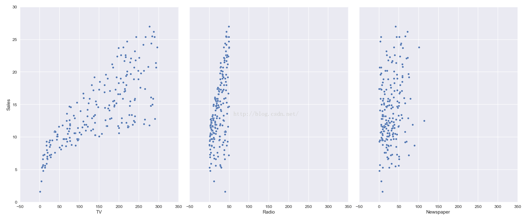
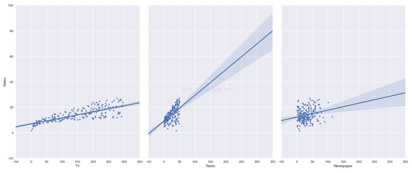
seaborn的pairplot函数绘制X的每一维度和对应Y的散点图。通过设置size和aspect参数来调节显示的大小和比例。可以从图中看出,TV特征和销量是有比较强的线性关系的,而Radio和Sales线性关系弱一些,Newspaper和Sales线性关系更弱。通过加入一个参数kind='reg',seaborn可以添加一条最佳拟合直线和95%的置信带。
结果显示如下:
4、线性回归模型
线性模型表达式: y=β0+β1x1+β2x2+...+βnxn 其中
- y是响应
- β0是截距
- β1是x1的系数,以此类推
在这个案例中: y=β0+β1∗TV+β2∗Radio+...+βn∗Newspaper
scikit-learn要求X是一个特征矩阵,y是一个NumPy向量。
pandas构建在NumPy之上。
因此,X可以是pandas的DataFrame,y可以是pandas的Series,scikit-learn可以理解这种结构。
输出结果如下:
TV Radio Newspaper 0 230.1 37.8 69.2 1 44.5 39.3 45.1 2 17.2 45.9 69.3 3 151.5 41.3 58.5 4 180.8 10.8 58.4 <class 'pandas.core.frame.DataFrame'> (200, 3)输出的结果如下:
0    22.1
1    10.4
2     9.3
3    18.5
4    12.9
Name: Sales
(2)、构建训练集与测试集
#default split is 75% for training and 25% for testing
输出结果如下:
输出的结果如下:
LinearRegression(copy_X=True, fit_intercept=True, normalize=False) 2.66816623043 [ 0.04641001 0.19272538 -0.00349015]
输出如下:
[('TV', 0.046410010869663267),
('Radio', 0.19272538367491721),
('Newspaper', -0.0034901506098328305)]
y=2.668+0.0464∗TV+0.192∗Radio-0.00349∗Newspaper
如何解释各个特征对应的系数的意义?
对于给定了Radio和Newspaper的广告投入,如果在TV广告上每多投入1个单位,对应销量将增加0.0466个单位。就是加入其它两个媒体投入固定,在TV广告上每增加1000美元(因为单位是1000美元),销量将增加46.6(因为单位是1000)。但是大家注意这里的newspaper的系数居然是负数,所以我们可以考虑不使用newspaper这个特征。这是后话,后面会提到的。
(4)、预测
输出结果如下:
[ 14.58678373 7.92397999 16.9497993 19.35791038 7.36360284 7.35359269 16.08342325 9.16533046 20.35507374 12.63160058 22.83356472 9.66291461 4.18055603 13.70368584 11.4533557 4.16940565 10.31271413 23.06786868 17.80464565 14.53070132 15.19656684 14.22969609 7.54691167 13.47210324 15.00625898 19.28532444 20.7319878 19.70408833 18.21640853 8.50112687 9.8493781 9.51425763 9.73270043 18.13782015 15.41731544 5.07416787 12.20575251 14.05507493 10.6699926 7.16006245 11.80728836 24.79748121 10.40809168 24.05228404 18.44737314 20.80572631 9.45424805 17.00481708 5.78634105 5.10594849] <type 'numpy.ndarray'>
5、回归问题的评价测度
(1) 评价测度
对于分类问题,评价测度是准确率,但这种方法不适用于回归问题。我们使用针对连续数值的评价测度(evaluation metrics)。
这里介绍3种常用的针对线性回归的测度。
1)平均绝对误差(Mean Absolute Error, MAE)
(2)均方误差(Mean Squared Error, MSE)
(3)均方根误差(Root Mean Squared Error, RMSE)
这里我使用RMES。
最后的结果如下:
<type 'numpy.ndarray'> <class 'pandas.core.series.Series'> 50 50 (50,) (50,) RMSE by hand: 1.42998147691(2)做ROC曲线
显示结果如下:(红色的线是真实的值曲线,蓝色的是预测值曲线)
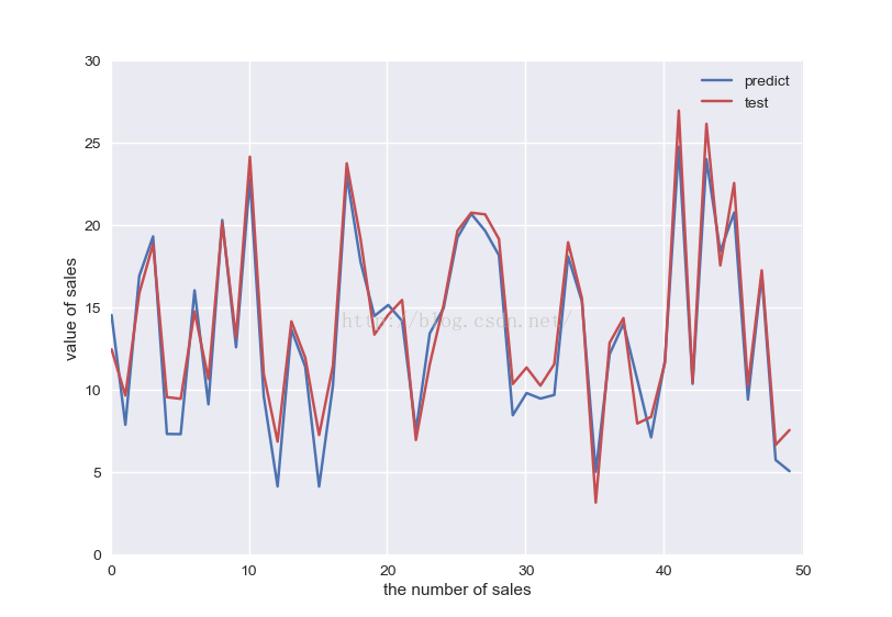
直到这里整个的一次多元线性回归的预测就结束了。
6、改进特征的选择
在之前展示的数据中,我们看到Newspaper和销量之间的线性关系竟是负关系(不用惊讶,这是随机特征抽样的结果。换一批抽样的数据就可能为正了),现在我们移除这个特征,看看线性回归预测的结果的RMSE如何?
依然使用我上面的代码,但只需修改下面代码中的一句即可:
# print the first 5 rowsprint X.head()# check the type and shape of Xprint type(X)print X.shape
最后的到的系数与测度如下:
LinearRegression(copy_X=True, fit_intercept=True, normalize=False)
2.81843904823 [ 0.04588771 0.18721008] RMSE by hand: 1.28208957507然后再次使用ROC曲线来观测曲线的整体情况。我们在将Newspaper这个特征移除之后,得到RMSE变小了,说明Newspaper特征可能不适合作为预测销量的特征,于是,我们得到了新的模型。我们还可以通过不同的特征组合得到新的模型,看看最终的误差是如何的。
备注:
之前我提到了这种错误:
ImportError                               Traceback (most recent call last)
<ipython-input-182-3eee51fcba5a> in <module>()
      1 ###构造训练集和测试集
----> 2 from sklearn.cross_validation import train_test_split
      3 #import sklearn.cross_validation
      4 X_train,X_test, y_train, y_test = train_test_split(X, y, random_state=1)
      5 # default split is 75% for training and 25% for testing

ImportError: cannot import name train_test_split
处理方法:1、我后来重新安装sklearn包。再一次调用时就没有错误了。
运算结果如下:
LinearRegression(copy_X=True, fit_intercept=True, normalize=False)
3.1066750253
[ 0.04588016  0.18078772 -0.00187699]
RMSE by hand: 1.39068687332


 3004
3004

 被折叠的 条评论
为什么被折叠?
被折叠的 条评论
为什么被折叠?
 到【灌水乐园】发言


