Caffe的各种层定义方法

1. Vision Layers

1.1 卷积层(Convolution)

类型：CONVOLUTION
例子

layer {
  name: "conv1"
  type: "Convolution"
  bottom: "data"
  top: "conv1"
  blobs_lr: 1
  blobs_lr: 2
  weight_decay: 1
  weight_decay: 0
  convolution_param {
    num_output: 96     # learn 96 filters
    kernel_size: 11    # each filter is 11x11
    stride: 4          # step 4 pixels between each filter application
    weight_filler {
      type: "gaussian" # initialize the filters from a Gaussian
      std: 0.01        # distribution with stdev 0.01 (default mean: 0)
    }
    bias_filler {
      type: "constant" # initialize the biases to zero (0)
      value: 0
    }
  }
}

blobs_lr: 学习率调整的参数，在上面的例子中设置权重学习率和运行中求解器给出的学习率一样，同时是偏置学习率为权重的两倍。
weight_decay：

卷积层的重要参数
必须参数：
num_output (c_o)：过滤器的个数
kernel_size (or kernel_h and kernel_w)：过滤器的大小

可选参数：
weight_filler [default type: ‘constant’ value: 0]：参数的初始化方法
bias_filler：偏置的初始化方法
bias_term [default true]：指定是否是否开启偏置项
pad (or pad_h and pad_w) [default 0]：指定在输入的每一边加上多少个像素
stride (or stride_h and stride_w) [default 1]：指定过滤器的步长
group (g)[default 1]: If g > 1, we restrict the connectivity of each filter to a subset of the input. Specifically, the input and output channels are separated into g groups, and the ith output group channels will be only connected to the ith input group channels.

通过卷积后的大小变化：
输入：n * c_i * h_i * w_i
输出：n * c_o * h_o * w_o，其中h_o = (h_i + 2 * pad_h - kernel_h) /stride_h + 1，w_o通过同样的方法计算。

1.2 池化层（Pooling）

类型：POOLING
例子

layer {
  name: "pool1"
  type: "Pooling"
  bottom: "conv1"
  top: "pool1"
  pooling_param {
    pool: MAX
    kernel_size: 3 # pool over a 3x3 region
    stride: 2      # step two pixels (in the bottom blob) between pooling regions
  }
}

重要参数:
必需参数：
kernel_size (or kernel_h and kernel_w)：过滤器的大小

可选参数：
pool [default MAX]：pooling的方法，目前有MAX, AVE, 和STOCHASTIC三种方法
pad (or pad_h and pad_w) [default 0]：指定在输入的每一遍加上多少个像素
stride (or stride_h and stride_w) [default1]：指定过滤器的步长

通过池化后的大小变化：
输入：n * c_i * h_i * w_i
输出：n * c_o * h_o * w_o，其中h_o = (h_i + 2 * pad_h - kernel_h) /stride_h + 1，w_o通过同样的方法计算。

1.3 Local Response Normalization (LRN)

类型：LRN
Local ResponseNormalization是对一个局部的输入区域进行的归一化（激活a被加一个归一化权重（分母部分）生成了新的激活b），有两种不同的形式，一种的输入区域为相邻的channels（cross channel LRN），另一种是为同一个channel内的空间区域（within channel LRN）
计算公式：对每一个输入除以

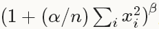
可选参数：
local_size [default 5]：对于cross channel LRN为需要求和的邻近channel的数量；对于within channel LRN为需要求和的空间区域的边长
alpha [default 1]：scaling参数
beta [default 5]：指数
norm_region [default ACROSS_CHANNELS]: 选择哪种LRN的方法ACROSS_CHANNELS 或者WITHIN_CHANNEL

2. Loss Layers

深度学习是通过最小化输出和目标的Loss来驱动学习。

2.1 Softmax

类型: SOFTMAX_LOSS

2.2 Sum-of-Squares / Euclidean

类型: EUCLIDEAN_LOSS

2.3 Hinge / Margin

类型: HINGE_LOSS
例子：

# L1 Norm
layer {
  name: "loss"
  type: "HingeLoss"
  bottom: "pred"
  bottom: "label"
}

# L2 Norm
layer {
  name: "loss"
  type: "HingeLoss"
  bottom: "pred"
  bottom: "label"
  top: "loss"
  hinge_loss_param {
    norm: L2
  }
}

可选参数：
norm [default L1]: 选择L1或者 L2范数
输入：
n * c * h * wPredictions
n * 1 * 1 * 1Labels
输出
1 * 1 * 1 * 1Computed Loss

2.4 Sigmoid Cross-Entropy

类型：SIGMOID_CROSS_ENTROPY_LOSS

2.5 Infogain

类型：INFOGAIN_LOSS

2.6 Accuracy and Top-k

类型：ACCURACY
用来计算输出和目标的正确率，事实上这不是一个loss，而且没有backward这一步。

3. 激励层（Activation / Neuron Layers）

一般来说，激励层是element-wise的操作，输入和输出的大小相同，一般情况下就是一个非线性函数。

3.1 ReLU / Rectified-Linear and Leaky-ReLU

类型: RELU
例子:

layer {
  name: "relu1"
  type: "ReLU"
  bottom: "conv1"
  top: "conv1"
}

可选参数：
negative_slope [default 0]:指定输入值小于零时的输出。

ReLU是目前使用做多的激励函数，主要因为其收敛更快，并且能保持同样效果。
标准的ReLU函数为max(x, 0)，而一般为当x > 0时输出x，但x <= 0时输出negative_slope。RELU层支持in-place计算，这意味着bottom的输出和输入相同以避免内存的消耗。

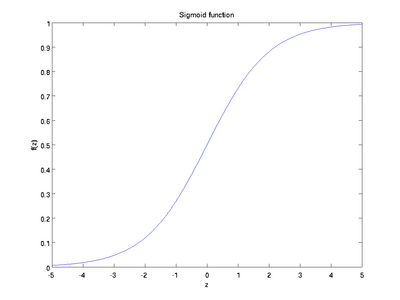
3.2 Sigmoid

类型: SIGMOID
例子:

layer {
  name: "encode1neuron"
  bottom: "encode1"
  top: "encode1neuron"
  type: "Sigmoid"
}

SIGMOID 层通过 sigmoid(x) 计算每一个输入x的输出，函数如下图。

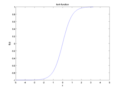
3.3 TanH / Hyperbolic Tangent

类型: TANH
例子:

layer {
  name: "layer"
  bottom: "in"
  top: "out"
  type: "TanH"
}

TANH层通过 tanh(x) 计算每一个输入x的输出，函数如下图。

3.4 Absolute Value

类型: ABSVAL
例子:

layer {
  name: "layer"
  bottom: "in"
  top: "out"
  type: "AbsVal"
}

ABSVAL层通过 abs(x) 计算每一个输入x的输出。

3.5 Power

类型: POWER
例子：

layer {
  name: "layer"
  bottom: "in"
  top: "out"
  type: "Power"
  power_param {
    power: 1
    scale: 1
    shift: 0
  }
}

可选参数：
power [default 1]
scale [default 1]
shift [default 0]
POWER层通过 (shift + scale * x) ^ power计算每一个输入x的输出。

3.6 BNLL

类型: BNLL
例子：

layer {
  name: "layer"
  bottom: "in"
  top: "out"
  type: BNLL
}

BNLL (binomial normal log likelihood) 层通过 log(1 + exp(x)) 计算每一个输入x的输出。

4. 数据层（Data Layers）

数据通过数据层进入Caffe，数据层在整个网络的底部。数据可以来自高效的数据库（LevelDB 或者 LMDB），直接来自内存。如果不追求高效性，可以以HDF5或者一般图像的格式从硬盘读取数据。

4.1 Database

类型：DATA
必须参数：
source:包含数据的目录名称
batch_size:一次处理的输入的数量

可选参数：
rand_skip:在开始的时候从输入中跳过这个数值，这在异步随机梯度下降（SGD）的时候非常有用
backend [default LEVELDB]: 选择使用 LEVELDB 或者 LMDB(较老版本没有)

layers {
  top: "data"
  top: "label_det"
  name: "data"
  type: DATA
  data_param {
    source: "imageset_test_leveldb"
    mean_file: "image_mean.binaryproto"
    batch_size: 1
     mirror: false
    crop_size: 0
     }
}

4.2 In-Memory

类型: MEMORY_DATA
必需参数：
batch_size, channels, height, width: 指定从内存读取数据的大小
The memory data layer reads data directly from memory, without copying it. In order to use it, one must call MemoryDataLayer::Reset (from C++) or Net.set_input_arrays (from Python) in order to specify a source of contiguous data (as 4D row major array), which is read one batch-sized chunk at a time.

4.3 HDF5 Input

类型: HDF5_DATA
必要参数：
source:需要读取的文件名
batch_size：一次处理的输入的数量

4.4 HDF5 Output

类型: HDF5_OUTPUT
必要参数：
file_name: 输出的文件名
HDF5的作用和这节中的其他的层不一样，它是把输入的blobs写到硬盘

4.5 Images

类型: IMAGE_DATA
必要参数：
source: text文件的名字，每一行给出一张图片的文件名和label
batch_size: 一个batch中图片的数量
可选参数：
rand_skip：在开始的时候从输入中跳过这个数值，这在异步随机梯度下降（SGD）的时候非常有用
shuffle [default false]
new_height, new_width: 把所有的图像resize到这个大小

layers {
  top: "data"
  top: "label_det"
  name: "data"
  type: IMAGE_DATA
  image_data_param {
    source: "test_root.txt"
    batch_size: 1
    mirror: false
    crop_size: 0
    mean_file: "image_mean.binaryproto"
  }
}

4.6 Windows

类型：WINDOW_DATA

4.7 Dummy

类型：DUMMY_DATA
Dummy 层用于development 和debugging。具体参数DummyDataParameter。

5. 一般层（Common Layers）

5.1 全连接层Inner Product

类型：INNER_PRODUCT
例子：

layer {
  name: "fc8"
  type: "InnerProduct"
  # learning rate and decay multipliers for the weights
  param { lr_mult: 1 decay_mult: 1 }
  # learning rate and decay multipliers for the biases
  param { lr_mult: 2 decay_mult: 0 }
  inner_product_param {
    num_output: 1000
    weight_filler {
      type: "gaussian"
      std: 0.01
    }
    bias_filler {
      type: "constant"
      value: 0
    }
  }
  bottom: "fc7"
  top: "fc8"
}

必要参数：
num_output (c_o)：过滤器的个数

可选参数：
weight_filler [default type: ‘constant’ value: 0]：参数的初始化方法
bias_filler：偏置的初始化方法
bias_term [default true]：指定是否是否开启偏置项

通过全连接层后的大小变化：
输入：n * c_i * h_i * w_i
输出：n * c_o * 1 *1

5.2 Splitting

类型：SPLIT
Splitting层可以把一个输入blob分离成多个输出blobs。这个用在当需要把一个blob输入到多个输出层的时候。

5.3 Flattening

类型：FLATTEN
Flattening是把一个输入的大小为n * c * h * w变成一个简单的向量，其大小为 n * (c*h*w) * 1 * 1。

5.4 Concatenation

类型：CONCAT

例子：

layer {
  name: "concat"
  bottom: "in1"
  bottom: "in2"
  top: "out"
  type: "Concat"
  concat_param {
    axis: 1
  }
}

可选参数：
concat_dim [default 1]：0代表链接num，1代表链接channels

通过全连接层后的大小变化：
输入：从1到K的每一个blob的大小n_i * c_i * h * w
输出：
如果concat_dim = 0: (n_1 + n_2 + … + n_K) c_1 h * w，需要保证所有输入的c_i 相同。
如果concat_dim = 1: n_1 * (c_1 + c_2 + … +c_K) * h * w，需要保证所有输入的n_i 相同。

通过Concatenation层，可以把多个的blobs链接成一个blob。

5.5 Slicing

The SLICE layer is a utility layer that slices an input layer to multiple output layers along a given dimension (currently num or channel only) with given slice indices.

layer {
  name: "slicer_label"
  type: "Slice"
  bottom: "label"
  ## Example of label with a shape N x 3 x 1 x 1
  top: "label1"
  top: "label2"
  top: "label3"
  slice_param {
    axis: 1
    slice_point: 1
    slice_point: 2
  }
}

5.6 Elementwise Operations

类型：ELTWISE

5.7 Argmax

类型：ARGMAX

5.8 Softmax

类型：SOFTMAX

5.9 Mean-Variance Normalization

类型：MVN

6. 参考

Caffe Tutorial