2021-10-01 深度学习之线性回归

综述

线性回归：其实就是一层神经网络
线性回归是对n维输入的加权，外加偏差
假设x是影响房价的因素，x可以是卫生间，居住面积等等，成交价就是y=w1x1+w2x2，w是权重，b是偏置。
y = w1x1+w2x1+…+b

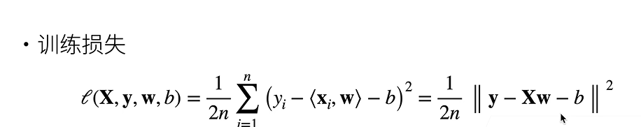
那么衡量预估质量，也就是房屋售价和估价的差距，也就是损失函数了。
这里利用均方误差：
**训练数据：**就是收集一些数据点来决定参数值，比如过去六个月卖的房子。

梯度下降

	在机器学习算法中，在最小化损失函数时，可以通过梯度下降法来一步步的迭代求解，得到最小化的损失函数，和模型参数值。反过来，如果我们需要求解损失函数的最大值，这时就需要用梯度上升法来迭代了。
	首先来看看梯度下降的一个直观的解释。比如我们在一座大山上的某处位置，由于我们不知道怎么下山，于是决定走一步算一步，也就是在每走到一个位置的时候，求解当前位置的梯度，沿着梯度的负方向，也就是当前最陡峭的位置向下走一步，然后继续求解当前位置梯度，向这一步所在位置沿着最陡峭最易下山的位置走一步。这样一步步的走下去，一直走到觉得我们已经到了山脚。当然这样走下去，有可能我们不能走到山脚，而是到了某一个局部的山峰低处。
	从上面的解释可以看出，梯度下降==不一定能够找到全局的最优解==，有可能是一个==局部最优解==。当然，==如果损失函数是凸函数，梯度下降法得到的解就一定是全局最优解==。
	![如图](https://img-blog.csdnimg.cn/9a4e3571c6034e0aa0c605d2401c4799.png?x-oss-process=image/watermark,type_ZHJvaWRzYW5zZmFsbGJhY2s,shadow_50,text_Q1NETiBA54ix5oqW6IW_55qE5bCP5p2-6byg,size_20,color_FFFFFF,t_70,g_se,x_16)
	步长（Learning rate）：步长决定了在梯度下降迭代的过程中，每一步沿梯度负方向前进的长度。用上面下山的例子，步长就是在当前这一步所在位置沿着最陡峭最易下山的位置走的那一步的长度。
	损失函数（loss function）：为了评估模型拟合的好坏，通常用损失函数来度量拟合的程度。损失函数极小化，意味着拟合程度最好，对应的模型参数即为最优参数。在线性回归中，损失函数通常为样本输出和假设函数的差取平方。

小批量随机梯度下降
随机采用b个样本来计算近似损失。batchsize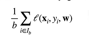
小批量随机梯度下降是深度学习默认的求解算法

线性回归从零开始实现的模型代码

import random
import torch
from d2l import torch as d2l

# 根据带有噪声的线性模型构造一个数据集，使用线性模型参数w = [2，-3.4]T，b=4.2和噪声生成数据集和标签
def synthetic_data(w,b,num_examples):
    "生成y = xw + b"
    x = torch.normal(0,1, (num_examples, len(w))) 
    #torch.normal(A, B ,size(C, D), 返回一个张量，requires_grad=True)A表示均值，B表示标准差 ,C代表生成的数据行数，D表示列数，requires_grad=True表示对导数开始记录，可以忽略。
    y = torch.matmul(x,w) + b  #torch.matmul是tensor的乘法，输入可以是高维的。当输入是都是二维时，就是普通的矩阵乘法，
    y = y + torch.normal(0 , 0.01, y.shape)  #减伤噪声
    print(x)
    print(len(x))
    return x, y.reshape((-1, 1))  #-1表示随便你换,但是列数必须是一列
      

true_w = torch.tensor([2, -3.4])
true_b = 4.2
features, labels = synthetic_data(true_w, true_b, 1000)
print(features[0])
print(labels[0])
"""
1、标签 label
即所要预测的结果是什么，如回归结果的y，分类问题中的分类结果，每一个类。
2.特征feature
事物的固有属性，做出判断的依据。如鸢尾花分类问题中，花瓣、花蕊等。一个事物具有N个特征，这些组成了事物的特性，作为机器学习中识别、学习的基本依据。
特征是机器学习的输入变量，如线性回归中的x。

"""

tensor([[-1.0894, -0.8842],
        [ 0.6656,  0.7123],
        [ 0.3343,  0.1520],
        ...,
        [ 0.9541,  1.2619],
        [ 0.2272, -0.2227],
        [-1.5065,  0.3997]])
1000
tensor([-1.0894, -0.8842])
tensor([5.0229])





'\n1、标签 label\n即所要预测的结果是什么，如回归结果的y，分类问题中的分类结果，每一个类。\n2.特征feature\n事物的固有属性，做出判断的依据。如鸢尾花分类问题中，花瓣、花蕊等。一个事物具有N个特征，这些组成了事物的特性，作为机器学习中识别、学习的基本依据。\n特征是机器学习的输入变量，如线性回归中的x。\n\n'

# features 中的每一行都有一个二维数据样本，labels每一行都包含一维标签值
print(features[0],labels[0])
print(features.shape)

tensor([-1.0894, -0.8842]) tensor([5.0229])
torch.Size([1000, 2])

d2l.set_figsize()
d2l.plt.scatter(features[:,1].detach().numpy(),
                labels.detach().numpy(),1)
#detach()分理处数值，不再含有梯度

<matplotlib.collections.PathCollection at 0x219593f8040>

[外链图片转存失败,源站可能有防盗链机制,建议将图片保存下来直接上传(img-EhH0V84M-1633084275934)(output_3_1.svg)]

# 定义一个data_iter 函数，这函数接收批量大小，特征矩阵和标签向量作为输入，生成batchsize的小批量
def data_iter(batch_size, features, labels):
    num_examples = len(features)
    indices = list(range(num_examples))
    #打乱样本，随机读取，没有特定顺序
    random.shuffle(indices)
    for i in range(0, num_examples, batch_size):
        batch_indices = torch.tensor(indices[i:min(i+batch_size,num_examples)])  # indices[1 : 11]
        yield features[batch_indices], labels[batch_indices] 
        


batch_size = 10
for x, y in data_iter(batch_size, features , labels):
    print(x, "\n" ,y)
    break


print(len(features))

tensor([[ 1.2411e+00, -6.2306e-05],
        [ 8.9213e-01, -8.8911e-01],
        [ 2.8689e-01,  1.9836e-01],
        [-1.2492e+00,  8.7085e-02],
        [ 1.2880e+00, -3.9923e-01],
        [ 3.6791e-02,  5.5911e-01],
        [ 1.4598e+00, -1.1351e+00],
        [-1.2349e+00, -7.4855e-01],
        [-3.3005e-02,  6.1077e-01],
        [-7.4842e-01,  1.0708e-01]]) 
 tensor([[ 6.6741],
        [ 9.0068],
        [ 4.1023],
        [ 1.4110],
        [ 8.1313],
        [ 2.3778],
        [10.9938],
        [ 4.2758],
        [ 2.0506],
        [ 2.3532]])
1000

# 定义初始化模型参数
w = torch.normal(0, 0.01, size=(2, 1), requires_grad=True)
b =torch.zeros(1, requires_grad=True)
print(w)
print(b)

tensor([[-0.0115],
        [ 0.0135]], requires_grad=True)
tensor([0.], requires_grad=True)

# 定义线性回归模型
def linreg(x, w ,b):
    "线性回归模型"
    return torch.matmul(x, w) + b

# 定义损失函数
def squared_loss(y_hat, y):
    "均方误差"
    return (y_hat - y.reshape(y_hat.shape))**2 / 2 

# 定义优化算法
def sgd(params, lr, batch_size):
    "小批量随机梯度下降"
    with torch.no_grad(): #更新的时候不要参与梯度计算，梯度存在于.grad中
        for param in params:
            param -=lr * param.grad / batch_size
            
            param.grad.zero_()  #把梯度设置成零，这样下一次计算梯度就不会和上一次相关了

# 训练过程

lr = 0.03
num_epochs = 3
net = linreg
loss = squared_loss

for epoch in range(num_epochs):
    print("epoch = {}".format(epoch))
    for x,y in data_iter(batch_size, features, labels):
        l = loss(net(x, w, b),y)  #计算x和y的小批量损失
        #计算关于w和b的梯度
        l.sum().backward()
        sgd([w,b],lr, batch_size)  #使用参数的梯度更新

    with torch.no_grad():
        train_l = loss(net(features, w, b),labels)
        print(f'epoch {epoch+ l}, loss{float(train_l.mean()):f}')

epoch = 0
epoch tensor([[0.0439],
        [0.0226],
        [0.0324],
        [0.0110],
        [0.0066],
        [0.0026],
        [0.1075],
        [0.0094],
        [0.1579],
        [0.2789]]), loss0.052127
epoch = 1
epoch tensor([[1.0000],
        [1.0002],
        [1.0006],
        [1.0001],
        [1.0000],
        [1.0000],
        [1.0000],
        [1.0000],
        [1.0002],
        [1.0000]]), loss0.000232
epoch = 2
epoch tensor([[2.0000],
        [2.0000],
        [2.0000],
        [2.0000],
        [2.0000],
        [2.0000],
        [2.0000],
        [2.0001],
        [2.0001],
        [2.0001]]), loss0.000049

2

线性回归的代码的简洁实现！

#线性回归的简洁，利用pytorch模块
from random import shuffle
import numpy as np
import torch
from torch.utils import data
from d2l import torch as d2l

true_w = torch.tensor([2, -3.4])
true_b = 4.2
features, labels = d2l.synthetic_data(true_w,true_b,1000)  # synthetic_data这个函数的作用就是之前我们辛苦编写的那几行代码，即y = xw+b

def load_array (data_arrays, batch_size, is_train=True):
    "构造一个pytorch迭代器"
    dataset = data.TensorDataset(*data_arrays)
    return data.DataLoader(dataset, batch_size, shuffle=is_train)

batch_size = 10
data_iter = load_array((features, labels),batch_size)

next(iter(data_iter))

[tensor([[ 2.4217,  1.6005],
         [ 0.5789, -0.5785],
         [ 2.1896, -0.8138],
         [-0.9653,  0.1172],
         [ 0.9881, -2.0501],
         [-0.2582,  0.0531],
         [-0.7596,  1.8117],
         [-0.5453, -0.5036],
         [ 0.4276,  0.0749],
         [ 1.8305,  0.5008]]),
 tensor([[ 3.6119],
         [ 7.3063],
         [11.3452],
         [ 1.8710],
         [13.1577],
         [ 3.5031],
         [-3.4791],
         [ 4.8220],
         [ 4.8098],
         [ 6.1526]])]

#模型的定义
from torch import nn
net = nn.Sequential(nn.Linear(2, 1))  # 线性模型 y = xw+b
net

Sequential(
  (0): Linear(in_features=2, out_features=1, bias=True)
)

net[0].weight.data.normal_(0, 0.01)
net[0].bias.data.fill_(0)

Sequential(
  (0): Linear(in_features=2, out_features=1, bias=True)
)

# 计算均方误差用mseloss
loss = nn.MSELoss()

# sgd 优化算法
trainer = torch.optim.SGD(net.parameters(), lr=0.03)

# 训练过程和我们从零开始很像
num_epochs = 3
for epoch in range(num_epochs):
    for x,y in data_iter:
        l = loss(net(x), y)
        
        trainer.zero_grad()
        l.backward()
        trainer.step()
        
    l = loss(net(features),labels)
    print(f'epoch{epoch+1}, loss{l:f}')
    

epoch1, loss0.000267
epoch2, loss0.000100
epoch3, loss0.000099