Solving PDE problem with ODE functions in MATLAB®

Solving PDE problem with ODE functions in MATLAB^®

PDE is Partial Differential Equation for short. Similarly, ODE is Ordinary Differential Equation for short. There are several ODE functions in MATLAB^®1 using numerical methods to approximate the result of ODE problems.

ODE functions in MATLAB

ODE functions in MATLAB are list as follow:

solver	Problem type	Order of Accuracy	When to use
ode45	Nonstiff	Medium	Most of the time. This should be the first solver you try.
ode15s	stiff	Low to medium	If ode45 is slow because the problem is stiff.

Table 1. ODE function list in MATLAB

Usage of ode45 and ode15s

As is illustrated in MATLAB help and documentations, ode45 and ode15s are similar in usage and basic structure, while the benefits and efficiency may differ when applied to different problems. The following is taking ode45 for instance, followed by comparison between ode45 and ode15s.

Basic structure of ode45

Basic structure of ode45 is

% basic structure of ode45 in MATLAB
[TOUT,YOUT] = ode45(ODEFUN,TSPAN,Y0);

An example is as follow:

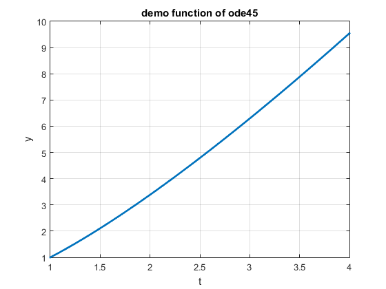
[t, y] = ode45(@func, [0 4], 1);

where func refer to a differential function

$$\begin{equation} \frac{\mathrm{d}y}{\mathrm{d}t}=\frac{y}{t}+1 \end{equation}$$
as is shown in MATLAB script

function dy = func(t, y)
% demo function of ode45
dy = y/t + 1; % function y with regard to t
end

Then, we plot this figure out.

Figure 1. Demo function of ode45

Let we think of some situation that parameters are given to ODEFUN. We take func for instance.
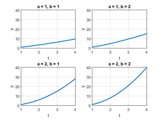
Consider the differential function with two parameters $a$ and $b$,

$$\begin{equation} \frac{\mathrm{d}y}{\mathrm{d}t}=a\frac{y}{t}+b \end{equation}$$
the function in MATLAB script is supposed to be

function dy = func(t, y, a, b)
% demo function of ode45
dy = a*y/t + b; % function y with regard to t
end

which calls for adapt to this function with parameters.

Parameter of ODEFUN in ode45

Let us look into ODEFUN in ode45 function, we can see the original usage of ODEFUN goes to @(t,y) func(t,y) which is shorted by @func with default no extra parameters. And in such case that parameters are demanded, we can use

[t, y] = ode45(@(t,y) func(t,y,a,b), [0 4], 1);

with a and b defined ahead.
And we can do parameter sweeping to see how parameters $a$ and $b$ influence the distribution of the differential function.

Figure 2. Parameter sweep of $a$ and $b$

Nonstiff and stiff problem

As is shown in Table 1, ode45 is applied to solve nonstiff problems, while ode15s is applied to solve stiff problems. So what is a stiff problem?

In mathematics, a stiff equation is a differential equation for which certain numerical methods for solving the equation are numerically unstable, unless the step size is taken to be extremely small. It has proven difficult to formulate a precise definition of stiffness, but the main idea is that the equation includes some terms that can lead to rapid variation in the solution. – [Wikipedia Stiff equation]

Thus we can see a nonstiff problem is the one that is not stiff. The following examples which is based on MATLAB documentation from Department of Radio Engineering, Czech Technical University will show the characteristic of nonstiff and stiff problems.

Nonstiff problem using ode45

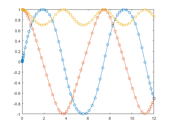
A typical example in MATLAB is rigidode, which is first illustrated in Shampine and Gordon’s book Computer Solution of Ordinary Differential Equations, 1975 solves the Euler equaions of a rigid body without external forces.

$$\begin{equation} \begin{cases} y_1'=y_2y_3, \\\\ y_2'=-y_1y_3, \\\\ y_3'=-0.51y_1y_2. \end{cases} \end{equation}$$
The solution of the ploblem is shown in rigidode in MATLAB. The simplified implement is as follow:

tspan = [0 12];
y0 = [0; 1; 1];
% solve the problem using ODE45
figure;
ode45(@f,tspan,y0);

function dydt = f(t,y)
dydt = [      y(2)*y(3)
             -y(1)*y(3)
        -0.51*y(1)*y(2) ];

As is shown in this MATLAB script, ode45 is used to solve this equation numerically. If we just type rigidode in MATLAB command line, the following figure will appear.

Figure 3. rigidode in MATLAB using ode45

Stiff problem using ode15s

Van der Pol equation is a typical stiff problem. The differential equations are as follow

⎧⎩⎨