凸优化（convex optimization）第二讲：convex set

Convex opt  第二讲（convex set）

Affine set

affine set 表示经过两点的一条线，这条线满足：

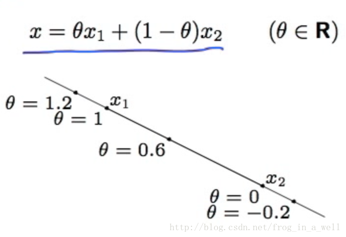
相较于后面我们要讨论的convex set，这里少了一些限制，是一个更广意义的直线，当theta取任意实数时，这条直线在无限的空间中延伸扩展。

当我们取theta大于1时，此时x1占的权重较大，x2较小，点就在靠近x1的方向上，当theta小于0时，此时x2占的权重较大，点就在靠近x2的方向上。

Affine set标准定义：

包含了所有经过affine set中任意两点的直线的set。

 

例子：什么是affineset：

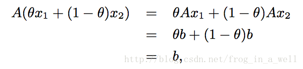
方程组的解空间。

如果我们有两个点可以解决上面的方程，那么他们的解的组合也是方程的解：推倒过程如下：

根据定义，我想在线性代数中的column space，row space，null space，left null space也是affine set，因为他们满足任意两个向量的线性组合也在这个space中。

Convex set

Convex set就是在affine set的基础之上多了一些条件，那条直线，变成了线段，我们通过限定theta的取值范围来限定set的取值为两点之间的线段。数学描述如下：

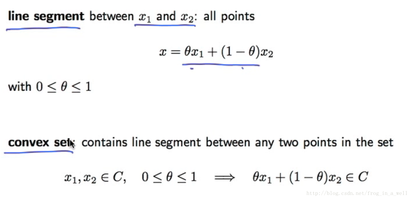
通过限定theta取值范围为0到1，我们能够得到：

反之亦然。

下面是一些关于convex set的例子：

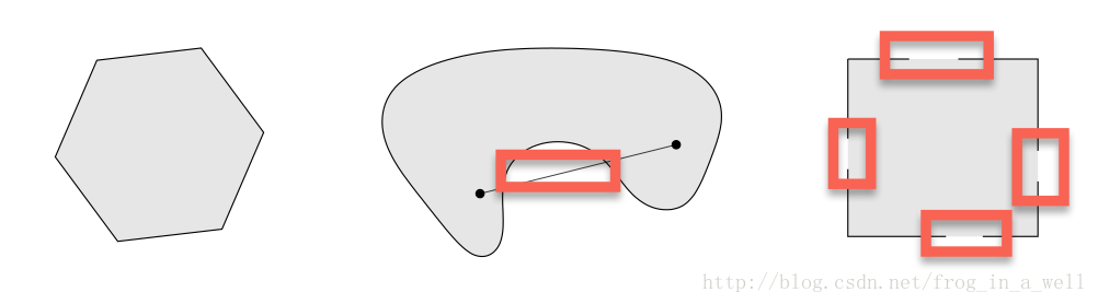
第一个图是一个正六边形，它是convex的，因为它内部的任意两点的连线也被包含在该图形的内部。

第二个图不是convex的，因为当我们连接set中的两点时，出现了未被包含在set中的点，即上图中红色方框中的区域。

第三个图不是convex的，原因同二。 

Convex combination

Convex combination是符合以下要求的形式：

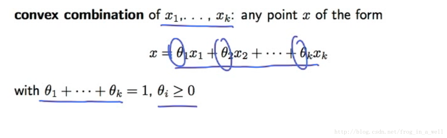
表示的是k个点以不同的权重相加生成一个新的点，权重是非负的，且theta相加之和为1。

Convex hull

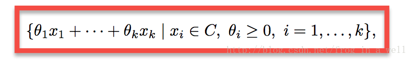
Convex hull 包含了set中所有点的convex combination组合出的所有的新点。其数学表示如下：

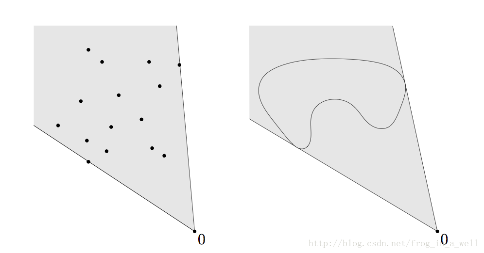
我们再来看看几何直观上的感受：

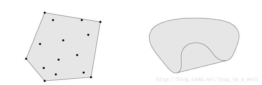
第一个图表示的是set中的点集通过convex combination过程形成的一个灰色区域，而这个区域就是convexhull。

第二个图是原来的肾形区域（non-convex）通过convex combination过程形成的另外一个灰色区域（convex）。

这个由基础点集生成一个convex空间的概念类似于线性代数中的column vector通过线性的运算来span column space。

那么convex hull的作用是什么呢？就是将non-convexset变成最小的包含原来non-convexset的convex set。

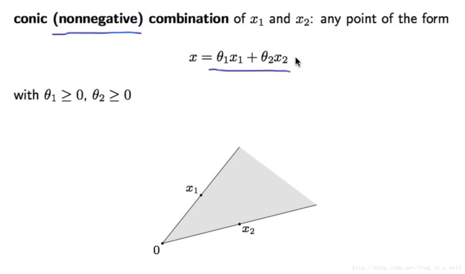
Conic combination

conic combination指的是由set中的任意两点通过线性组合产生一个新点，线性组合是非负的。

几何意义是一个通过vectorx1，x2产生锥形区域。在线性代数中即为两个vector的线性组合生成的空间中非负组合的那一块。

Conic cone

Conic cone是包含原来set中所有点经过conic combination组合产生的点的set。

这个set对应至前面我们的affineset-convex set- convex hull概念链条中的affine set，是一个比较general的概念。

Conic hull

conic hull是包含了原来set中所有点的最小的conic cone。

 

例子：以下是两个conichull的例子：coniccone可以想象为在以下的hull基础上增加了一些元素。

 

一些重要的例子

通过之前的定义，我们不难得出以下结论：

1.    空集和包含一个点的点集是affine且convex的。

2.    一条直线是affine的，如果这条线过原点，那么它还是convex cone。

3.    一条线段是convex的，但不是affine的（除非其为一个点）。

4.    一条射线是convex的，但不是affine的。

5.    任何的subspace是affine的，也是convex cone。

超平面和半空间

关于超平面，这里有详细的讲解：http://bubblexc.com/y2011/310/

这里要注意的是a和b的值，通过调整b的值我们可以调整超平面距离原点的距离，调整a的值来调整超平面的方向。

超平面是affine和convex的。

半空间是将超平面中的等式改变为不等式，用所确定的超平面来分离空间，使之成为两个半空间。

半空间是convex的，但不是affine的。

欧拉球和椭球

欧拉球：

表示为离中心点距离小于等于r（半径）的点的集合，数学表示如下：

当然也能表示成另外一种形式：中心点加上一个norm小于1的向量的r倍。

椭球

椭球的公式如下：

P是一个对称正定矩阵，椭球的轴长，由正定矩阵的的特征值的平方根给出。

另外一种表示方式是：

unit ball经过线性变换加上改变中心点形成了一个椭球。

Norm balls and norm cones

norm是一种function的表示，这种function有以下性质：

1．        x的norm大于等于0，当且仅当x=0时，x的norm等于0。

2．        一个向量x的t倍的norm等于t倍的x的norm

3．        两个向量的norm符合三角不等定理，其几何意义如有上图的平行四边形法则。

Norm外面的symb表示的是symb次方的symb次根。

Norm ball 和norm cone

Norm ball表示的是离center点一定距离r的点。

Norm cone表示的是norm的值小于t的点，对于二维的平面，随着t的增大，圆形是逐渐变大的，见下面的圆锥体即为二维平面的normcone。

norm cone是convex的。

Polyhedra 多面体

Polyhedral在几何上的意义是表示有限个线性不等式或等式的解的可行域，数学表示如下：

要注意的是A是m*n个元素的矩阵，表示的是m个不等式，每个不等式中有n个元素（constrain variable）。C表示p个含有n个限制变量的等式。以及挨个元素对比大小的符号，是表示比较两个vector中的每个元素的大小。

其中Ax中的每一行表示的是一个超平面，每个不等式表示的是一个半空间，而整个可行的区域是由以上的等式和不等式共同决定的，就是这些半空间（不等式）和超平面（等式）交集。这些都是线性规划的内容。

Positive semidefinite cone

S表示的是对称的矩阵，下面如果有+号，表示的是对称半正定矩阵，如果有两个加号就是对称正定矩阵。

下图示例展示了一个半正定矩阵确定的cone：

关于用矩阵来表示二次多项式，有如下形式：

对应至二次多项式，上图中的条件就好理解了，具体的推导可以参见gilbert strang的《Linear Algebra and Its Applications 4ed》第344页。 

对应至多维的是这样：

 

operations that preserve convexity 保持凸性的运算

交集

有限个凸集的交集一定是凸集。扩展至无限多的凸集也一样，

例子：

多边形是有限个半空间和超平面的交集，因为半空间和超平面是凸的，那么多边形也是凸的。 

所有的凸集S都是一系列半空间的交集。数学表示如下：

例子：

对于上例，我们可以将p（t）看做是两个vector的内积，一个vector是x，另外一个是coskt，那么这样一个内积确定的超平面的绝对值小于1，即p（t）小于等于1，大于等于负1。P（t）小于等于1确定了一个半空间，大于等于负1确定了另外一个半空间（halfspace），最终我们得到的是两个半空间的交集，因为半空间是凸的，所以我们得到的最终结果也是凸的。其几何意义表示如下：

上图可以看出最终的区域是所有满足不等式的vectorx所确定的半空间的交集，即为中间区域S，是convex的。

Affine function 仿射函数

将n维的convexset映射至m维的运算结果也是convex的。

一个通过映射得到的convexset，它的反函数也是convexset。

以下运算也可以保持凸性：

scaling

translation

projection

透视函数

透视函数的直观理解如下：x3=0为一个不透光隔板，只有在原点有一个小孔，光透过小孔投射至x3=-1的隔板上，如果上面的光点所构成的set是convex的，那么投射至下方的光点构成的set也是convex的。更加直观的想象我们通过一个针孔照相机去拍摄一个convex的对象，那么生成的图像也是convex的。

数学描述如下：

  

generalized inequality

proper cones

当K满足如下条件，我们说K是proper cone

我们用这样的proper cone来定义generalize inequality。

y大于等于x，表示成为y与x的差值属于一个proper cone K。

如果y严格大于x，那么表示成为以下：

对于矩阵的元素间的比较，有：

 

generalized inequality 属性

以上的比较全为vector间的元素比较。

加持性：y大于x，v大于u，那么y+v大于x+u。

传递性：y大于x，z大于y，那么z大于x。

非负scaling：y大于x，a大于0，那么a*x小于a*y。

反身性：x小于等于x中的元素。

反对称性：如果x大于等于y，y大于等于x，那么x等于y。

极限保持性：如果xi小于等于yi，对于i等于1，2，3知道无穷大都成立，那么x小于等于y。

 

对于严格小于，有以下性质：

 

极小值和最小值：

符号≼，≺是继承至传统的小于符号，我们已经在上面看到了不少传统的大小比较性质可以直接继承用来方便我们的表示，但是有些性质就不能适用了，比如传统的比较是线性的排序，任何的两个元素都是可比较的，比如两个元素x，y，要不就是x大于等于y，要不就是y大于等于x，总能分出个胜负，但是当我们用于generalized inequality时，大小就不那么明显了。

Minimum

Minimum的定义如下：

S中的任意一点y都大于等于x，那么x就是S中的minimum点。Minimum我们一般认为是最小值点，即在一个set中是唯一的。但是minimal极小值点可以是多个的。

Minimal

极小值minimal的定义如下：

极小值就是在S中找不出来小于或者等于x却又不是x的元素。

用传统的表示方法如下：

对于最小值x，有：

这里的x+K表示的是所有大于等于x的值，K是proper cone。

对于极小值x，有：

表示的是所有小于x的值与S的交集只有x自己。

对于最小值minimum和极小值minimal的直观表示如下：

左边的图深色区域表示的是convexset S1，浅灰色区域是最小值+K，那么我们的任务是从S1中找出一个点使得S1中所有的点都大于等于它，这个点就是x1.右边的图深色区域表示的是convexset S2,浅灰色区域是x-K，即小于x的值，根据定义小于极小值的值与S的交点只有极小值，那么极小值就是x2。这里我们发现极小值并不唯一，因为当我们取x2所在直线边缘的其他点，也满足这样的要求。

Separating hyperplane theorem 超平面分割理论

Separating hyperplane

对于两个在空间中不相交的set，我们总能找到合适的超平面来分割它们，图形如下所示：

严格的分割面只是将上述的大于等于或者小于等于符号换成大于或者小于。

Support hyperplanes

支持超平面就是经过set边缘的超平面，对于convex set，在set的边缘的每一点都有这样的支持超平面。

 

这里要注意的是有些点的支持超平面不唯一，特别是像一些不可导的点，想象下正方形的四个角。

dual cone and generalized inequality

dual cone

dual cone的定义如下：假设x属于一个cone K，那么dual cone就是那些与所有x相乘大于等于0的向量所构成的cone。

直观的感受如下：

左图的y与K中的所有向量的夹角小于90度，所以根据乘积法则，它们的乘积始终大于0，所以y属于K的dual cone中的一员。右图的z与K中的部分向量的夹角大于90度，所以部分的乘积小于0，则z不属于k的dual cone。So，我们画出它的dual cone是如下样子滴，两条红线所夹的区域两条红色的线是分别与K的边界成90度的线，如果大于了90度就会出现与原来的cone乘积小于0的情况。

所以我们可以想象一下，如果original cone K是比较苗条的，那么dual cone 就比较粗胖。如果original cone是二维空间的一个half space，那么dual cone就是一条与分割超平面垂直的向量。

下面是一些例子：

如果K是第一象限，那么其dualcone 也是第一象限，推广至任何成90度的cone的dualcone都是它们自身，这也叫做自身对偶性。

半正定矩阵的dualcone也是半正定矩阵。

 

 

 References：

1. Convex Optimization Boyd and Vandenberghe

2. convex optimization 101 by Boyd