gradient checking（梯度检验）

Gradient Checking（梯度检验）

我们有时候实现完backward propagation，我们不知道自己实现的backward propagation到底是不是完全正确的（这篇博客只面向自己手撸的网络，直接搬砖的不需要考虑这个问题…），因此，通常要用梯度检验来检查自己实现的bp是否正确。其实所谓梯度检验，就是自己实现下导数的定义，去求w和b的导数（梯度），然后去和bp求到的梯度比较，如果差值在很小的范围内，则可以认为我们实现的bp没问题。

先来回顾下，导数的定义：

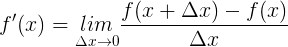
具体应用到神经网络的梯度检验中，因为我们没法做到$\Delta x\to 0$，只能取一个比较小的数，所以为了结果更精确，我们可以把上面的公式稍微变下形：

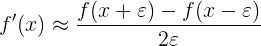
通常设置 $\epsilon =e^{-7}$即可。
具体到神经网络中，我们做梯度检验的步骤通常为：

1. 把 $W^{[1]},b^{[1]},......,W^{[L]},b^{[L]}$ 转化成向量 $\theta$。
2. 同样把 $d{W}^{[1]},d{b}^{[1]},......,d{W}^{[L]},d{b}^{[L]}$ 转化成向量 $d\theta$。
3. 接下来是实现导数定义：

4. 接下来我们比较 $d{\theta }_{approx}$ 与 $d\theta$ 是否大致相等，主要是计算两个向量之间的欧式距离：

通常设置阈值 $threshold=e^{-7}$。 如果difference小于阈值，则认为实现的bp没问题。


关于上面的步骤，我们来看看代码实现，

1.把 $W^{[1]},b^{[1]},......,W^{[L]},b^{[L]}$ 转化成向量 $\theta$。

#convert parameter into vector
def dictionary_to_vector(parameters):
	"""
	Roll all our parameters dictionary into a single vector satisfying our specific required shape.
	"""
	count = 0
	for key in parameters:
		# flatten parameter
		new_vector = np.reshape(parameters[key], (-1, 1))#convert matrix into vector
		if count == 0:#刚开始时新建一个向量
			theta = new_vector
		else:
			theta = np.concatenate((theta, new_vector), axis=0)#和已有的向量合并成新向量
		count = count + 1

	return theta

2.把 $d{W}^{[1]},d{b}^{[1]},......,d{W}^{[L]},d{b}^{[L]}$ 转化成向量 $d\theta$。
注：这个地方一定要注意bp求得的gradients字典的存储顺序是{dWL,dbL,…dW2,db2,dW1,db1}，因为后面要求欧式距离，所以一定要把顺序转化为[dW1,db1,…dWL,dbL]。在这个地方踩过坑，花了很长时间才找出bug。

#convert gradients into vector
def gradients_to_vector(gradients):
	"""
	Roll all our parameters dictionary into a single vector satisfying our specific required shape.
	"""
	# 因为gradient的存储顺序是{dWL,dbL,....dW2,db2,dW1,db1}，
	#为了统一采用[dW1,db1,...dWL,dbL]方面后面求欧式距离（对应元素）
	L = len(gradients) // 2
	keys = []
	for l in range(L):
		keys.append("dW" + str(l + 1))
		keys.append("db" + str(l + 1))
	count = 0
	for key in keys:
		# flatten parameter
		new_vector = np.reshape(gradients[key], (-1, 1))#convert matrix into vector
		if count == 0:#刚开始时新建一个向量
			theta = new_vector
		else:
			theta = np.concatenate((theta, new_vector), axis=0)#和已有的向量合并成新向量
		count = count + 1

	return theta

第三步、第四步的代码如下：

def gradient_check(parameters, gradients, X, Y, layer_dims, epsilon=1e-7):
	"""
	Checks if backward_propagation_n computes correctly the gradient of the cost output by forward_propagation_n

	Arguments:
	parameters -- python dictionary containing your parameters "W1", "b1", "W2", "b2", "W3", "b3":
	grad -- output of backward_propagation_n, contains gradients of the cost with respect to the parameters.
	x -- input datapoint, of shape (input size, 1)
	y -- true "label"
	epsilon -- tiny shift to the input to compute approximated gradient with formula(1)
	layer_dims -- the layer dimension of nn
	Returns:
	difference -- difference (2) between the approximated gradient and the backward propagation gradient
	"""

	parameters_vector = dictionary_to_vector(parameters)  # parameters_values
	grad = gradients_to_vector(gradients)
	num_parameters = parameters_vector.shape[0]
	J_plus = np.zeros((num_parameters, 1))
	J_minus = np.zeros((num_parameters, 1))
	gradapprox = np.zeros((num_parameters, 1))

	# Compute gradapprox
	for i in range(num_parameters):
		thetaplus = np.copy(parameters_vector)
		thetaplus[i] = thetaplus[i] + epsilon
		AL, _ = forward_propagation(X, vector_to_dictionary(thetaplus,layer_dims))
		J_plus[i] = compute_cost(AL,Y)

		thetaminus = np.copy(parameters_vector)
		thetaminus[i] = thetaminus[i] - epsilon
		AL, _ = forward_propagation(X, vector_to_dictionary(thetaminus, layer_dims))
		J_minus[i] = compute_cost(AL,Y)
		gradapprox[i] = (J_plus[i] - J_minus[i]) / (2 * epsilon)

	numerator = np.linalg.norm(grad - gradapprox)
	denominator = np.linalg.norm(grad) + np.linalg.norm(gradapprox)
	difference = numerator / denominator

	if difference > 2e-7:
		print(
			"\033[93m" + "There is a mistake in the backward propagation! difference = " + str(difference) + "\033[0m")
	else:
		print(
			"\033[92m" + "Your backward propagation works perfectly fine! difference = " + str(difference) + "\033[0m")

	return difference

这里在每一次计算bp时，还要把向量转化成矩阵，具体实现如下：

#convert vector into dictionary
def vector_to_dictionary(theta, layer_dims):
	"""
    Unroll all our parameters dictionary from a single vector satisfying our specific required shape.
    """
	parameters = {}
	L = len(layer_dims)  # the number of layers in the network
	start = 0
	end = 0
	for l in range(1, L):
		end += layer_dims[l]*layer_dims[l-1]
		parameters["W" + str(l)] = theta[start:end].reshape((layer_dims[l],layer_dims[l-1]))
		start = end
		end += layer_dims[l]*1
		parameters["b" + str(l)] = theta[start:end].reshape((layer_dims[l],1))
		start = end
	return parameters

还是拿sklearn中自带的breast_cancer数据集，来测试下，自己实现的bp到底对不对，顺便也是测下我们的gradient checking的代码对不对，测试结果如下： >Your backward propagation works perfectly fine! difference = 5.649104934345307e-11

可以看到我们实现的bp求到的梯度和用导数定义实现的梯度之间的差距是$e^{-11}$这个数量级，所以我们实现的bp正确无误。
完整的代码已放到github上：gradient_checking.py


cs231n中也有讲解关于gradient cheking的资料，不过它的$relativeerror$ 定义和ng讲的有些细微的差别，不过不是什么大问题，只是定义不一样而已，只要改变相应的阈值即可。具体见：CS231n Convolutional Neural Networks for Visual Recognition

参考资料 - ng Coursera 《Improving Deep Neural Networks Hyperparameter tuning, Regularization and Optimization》课