python积铢累寸

一、python package

1.numba

numba有两种编译模式：nopython模式和object模式。前者能够生成更快的代码，但是有一些限制可能迫使numba退为后者。想要避免退为后者，而且抛出异常，可以传递nopython=True.

import numba
@jit(nopython=True)
def f(x, y):
    return x + y

numba目标是加快面向数组的计算，可使用它们库中提供的函数来解决。需要说明的是，numba库也有很多函数是不能用的（这个后续会整理）。
numba更多功能请参考：https://www.jianshu.com/p/4eb221c9bf55

2 pandas

2.1 向量操作

有一组数据，需要实现如下功能："Time"是日期-时分秒的格式，现在要求把"Time"拆为日期和时分秒两列，“day"和"hhmmss”。

 import pandas as pd
   column = ['Time', 'val1', 'val2', 'val3', 'val4']
    data = [['20190603-09:41:45', 11, 8, 17.12, 7.7],
            ['20190603-09:41:48', 12, 9.2, 12.23, 3.6],
            ['20190603-09:41:51', 12, 9.3, 15.13, 5.8],
            ['20190603-09:41:54', 13, 3.4, 11.9, 2.4],
            ['20190603-09:41:57', 14, 2.6, 9.3, 3.7],
            ['20190603-09:42:32', 15, 3.0, 6.5, 13.5],
            ['20190603-10:01:02', 11, 2.5, 2.22, 9.4]]
    print(data)
    df = pd.DataFrame(data=data, columns=column)

采用iloc，iterrows、itertuple、apply实现上述功能，并对其进行性能比较。

2.1.1 iloc

显然，用iloc或者loc逐行遍历，然后用正则匹配即可达到效果，代码如下：
def iloc_loop(df):
# 逐行遍历df，以’-'为分隔符将字符串split

  day_lis = []
    time_lis = []
    for i in range(len(df)):
        str_split = df.iloc[i]['Time'].split('-')
        day_lis.append(str_split[0])
        time_lis.append(str_split[1])
    df['day'] = day_lis
    df['hhmmss'] = time_lis
    print(df)

2.1.2 iterrows

用iterrows逐行访问
代码如下：

def use_iterrows(df):
    day_lis = []
    time_lis = []

# 将iloc定位行改为iterrows遍历    for index, row in df.iterrows():

    str_split = row['Time'].split('-')
        day_lis.append(str_split[0])
        time_lis.append(str_split[1])
    df['day'] = day_lis
    df['hhmmss'] = time_lis
    print(df)

2.2.3 itertuples

也可用itertuples实现
代码如下：

def use_itertuples(df):                       
    day_lis = []                              
    time_lis = []                             
    # 将iloc定位行改为iterrows遍历                    
    for row in df.itertuples():               
        # print('index=', row[1])             
        str_split = row[1].split('-')         
        day_lis.append(str_split[0])          
        time_lis.append(str_split[1])         
    df['day'] = day_lis                       
    df['hhmmss'] = time_lis                   
    return df       

三种处理方式的性能比较如下

显然，iterrows 和itertuples效率更高。

2.2.4 apply 函数

利用apply函数也可实现上述功能。

def try_apply(df):
      df['day'] = df['Time'].apply(lambda x: x.split('-')[0])
      df['hhmmss'] = df['Time'].apply(lambda x: x.split('-')[1])
try_apply(df)

执行时间结果如下：

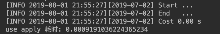
使用apply()函数让代码变得更简洁、易读，并且耗时大幅减小至0.0009S！这是因为apply函数对传入的参数进行了并行化处理，使处理效率大大提升.

2.2.5 isin()

有一组数据，需要将小时按照区间划分，每个区间乘以不同的参数值作为新值

def apply_tariff_isin(df):
    # 定义小时范围Boolean数组
    peak_hours = df.index.hour.isin(range(17, 24))
    shoulder_hours = df.index.hour.isin(range(7, 17))
    off_peak_hours = df.index.hour.isin(range(0, 7))
    # 使用上面的定义
    df.loc[peak_hours, 'cost_cents'] = df.loc[peak_hours, 'energy_kwh'] * 28
    df.loc[shoulder_hours,'cost_cents'] = df.loc[shoulder_hours, 'energy_kwh'] * 20
    df.loc[off_peak_hours,'cost_cents'] = df.loc[off_peak_hours, 'energy_kwh'] * 12

run一下，观察一下运行时长

>>> apply_tariff_isin(df)
Best of 3 trials with 100 function calls per trial:

Function apply_tariff_isin ran in average of 0.010 seconds.
.isin()方法返回的是一个布尔值数组
结果如下：
[False, False, False, …, True, True, True]
从这一点上看，发现仍然有性能提升，但它本质上变得更加边缘化。

2.2.6 cut

2.2.5需要实现的逻辑，上述操作也可通过cut完成，代码如下
def apply_tariff_cut(df):
# pd.cut() 根据每小时所属的bin应用一组标签(costs)
cents_per_kwh = pd.cut(x=df.index.hour,
bins=[0, 7, 17, 24],
include_lowest=True,
labels=[12, 20, 28]).astype(int)
df[‘cost_cents’] = cents_per_kwh * df[‘energy_kwh’]
run一下，观察一下运行时长

>>> apply_tariff_cut(df)
Best of 3 trials with 100 function calls per trial:
Function `apply_tariff_cut` ran in average of 0.003 seconds.

使用numpy的 digitize() 也可实现上述操作
它类似于Pandas的cut()，数据将被分箱，但这次它将由一个索引数组表示，这些索引表示每小时所属的bin。然后将这些索引应用于价格数组。

def apply_tariff_digitize(df):
    prices = np.array([12, 20, 28])
    bins = np.digitize(df.index.hour.values, bins=[7, 17, 24])
    df['cost_cents'] = prices[bins] * df['energy_kwh'].values

观察一下运行时长

>>> apply_tariff_digitize(df)
Best of 3 trials with 100 function calls per trial:
Function `apply_tariff_digitize` ran in average of 0.002 seconds

从这一点看，发现仍然有性能提升，但它本质上变得更加边缘化

2.2 stack

stack具有逆透视的功能，通俗地讲，即将列名转换为普通的列
有如下一组数据

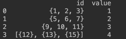
需要将其转换为如下格式

初步思路是，先进行一步正则化操作，然后利用stack,将该列名转化为普通的列
代码如下：

df.set_index('value',inplace=True)
df['id']= df['id'].apply(lambda x:str(x)).apply(lambda x:re.sub('{|}|\[|\]','',x))
df= df['id'].str.split(',',expand=True).stack().reset_index(level=1, drop=True).reset_index(drop=False)
df.rename(columns={0:'id'}, inplace = True)

世欢版

from itertools import chain
tmp_df = pd.DataFrame()
df['id'] = df['id'].apply(lambda x: list(chain(*x)) if isinstance(x, list) else x)
tmp_df['id'] = list(chain(*df['id']))
tmp_df['value'] = list(chain(*[[j]*i for i,j in zip(df['id'].apply(len), df['value'])]))

两版本时间复杂度对比

2.3 agg

对分组后的部分列进行聚合，并修改列名

import pandas as pd
df = pd.DataFrame({'Country': ['China', 'China', 'India', 'India', 'America', 'Japan', 'China', 'India'],
 'Income': [10000, 10000, 5000, 5002, 40000, 50000, 8000, 5000], 'Age': [5000, 4321, 1234, 4010, 250, 250, 4500, 4321]})
print(df)
df_agg = df.groupby('Country').agg({'Age':['min', 'mean', 'max'],'Income':['min','max']})
col = ['_'.join(col).strip() for col in df_agg.columns.values]
df_agg.columns = col
print(df_agg)

运行结果如下：

2.3.1 调用多个聚合函数#对函数加元祖，添加新的列名

按照某一列进行分组，获取DataFrame中某一分组的数据的最大值和最小值之差

lis = [[6,3,'a','one'],
       [5,8,'b','one'], 
       [8,7,'a','two'], 
       [1,2,'b','three'],  
       [4,6,'a','two'],   
       [5,4,'b','two'],  
       [1,7,'a','one'],  
       [3,9,'a','three']]
df = pd.DataFrame(data = lis,columns=['vec1','vec2','vec3','vec4'])
print(df)

• 自定义函数实现

def peak_range(df):
    return df.max()-df.min()
tmp= df.groupby('vec3').agg(peak_range)
print(tmp)

• lambda实现
  tm= df.groupby(‘vec3’).agg(lambda x:x.max()-x.min())
  print™

• 调用多个聚合函数#对函数加元祖，添加新的列名

tmp =df.groupby('vec3').agg(['mean','std','count',('pt',peak_range)])
print(tmp)

结果如下

2.4 rolling

pandas的rolling函数用来计算时间窗口数据
函数原型为：

DataFrame.rolling(window, min_periods=None, center=False, win_type=None, on=None, axis=0, closed=None)

DataFrame.rolling(window, min_periods=None, center=False, win_type=None, on=None, axis=0, closed=None)
arr = np.array([[2,2,2], [4,4,4], [6,6,6], [8,8,8], [10,10,10]])
df2 = pd.DataFrame(arr, columns = ['one', 'two', 'three'], 
                  index = pd.date_range('1/1/2018', periods = 5))

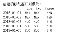
print(‘创建的移动窗口对象为：\n’, df2.rolling(3).mean())
结果如下：

print('创建的移动窗口对象为：\n', df2.rolling(3,min_periods=2).mean())

结果如下：

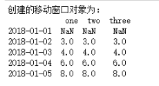
其中，min_periods表示窗口最少包含的观测值，小于这个值的窗口长度显示为空，等于和大于时有值，如上面结果所示：min_periods=2，表示窗口最少包含的观测值为2，所以2018-01-01没有值

2.5 to_datetime()

pd.to_datetime()是一个很好的时间转换工具,但是函数虽好，如果不注意细节会存在耗时问题，如使用format和不使用format耗时就不一样。如下：
数据如下

index,date_time
1,2019-08-07 23:59:59
2,2019-08-05 23:59:59
3,2019-08-07 23:59:59
4,2019-08-07 23:59:59
5,2019-08-07 23:59:59
6,2019-08-07 23:59:59
7,2019-08-05 23:59:59
8,2019-08-07 23:59:59
9,2019-08-05 23:59:59
10,2019-08-07 23:59:59
11,2019-08-05 23:59:59
12,2019-08-07 23:59:59
13,2019-08-05 23:59:59

”“”
代码如下

df = pd.read_csv('sx.csv')
print(df)
df1 = df.copy()
start = time.time()
df1['date_time'] = pd.to_datetime(df1['date_time'])
end=time.time()
print('time no use format=',end-start)
df1 = df.copy()
start = time.time()
format='%Y-%m-%d %H:%M:%S'
df1['date_time']= pd.to_datetime(df1['date_time'],format=format)
end=time.time()
print('time use format=',end-start)

结果如下：

也可采用自定义函数，在read_csv的文件头中调用
代码如下：

start = time.time()
dateparse = lambda dates: pd.datetime.strptime(dates, '%Y-%m-%d %H:%M:%S')
df = pd.read_csv('sx.csv',date_parser=dateparse,parse_dates=True,index_col='date_time')
end=time.time()
print('parse time=',end-start)

消耗时间为：
由此可知，在文件头调用自定义函数所耗时间更长

2.6 cumsum()

cumsum函数：计算轴向元素累积加和的数据
axis可取0，1。axis等于几，就是在那个轴累计求和
cumsum用法如下：
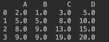
当axis=0时，代码如下

import pandas as pd
fs = pd.DataFrame([[2.0, 1.0,3.0,5],
                   [3.0, 4.0,5.0,5],
                   [3.0, 4.0,5.0,5],
                   [1.0, 0.0,6.0,5]],
columns = list('ABCD'))
print(fs.cumsum(axis=0))

结果如下

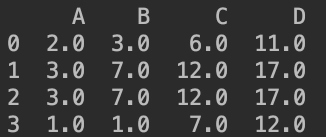
当axis=1时，代码如下

print(fs.cumsum(axis=1))

结果如下：

拓展：numpy 的cumsum

arr =np.array([[[1,2,3],[8,9,12]],[[1,2,4],[2,4,5]]])#2*2*3
print(arr.cumsum(0))
print("\n")
print(arr.cumsum(1))
print("\n")
print(arr.cumsum(2))
print("\n")

结果如下：

2.7 pd.crosstab()

交叉表是用于统计分组频率的特殊透视表
** 参数**

index : array-like, Series, or list of arrays/Series 
Values to group by in the rows
columns : array-like, Series, or list of arrays/Series 
Values to group by in the columns
values : array-like, optional 
Array of values to aggregate according to the factors
aggfunc : function, optional 
If no values array is passed, computes a frequency table
rownames : sequence, default None 
If passed, must match number of row arrays passed
colnames : sequence, default None 
If passed, must match number of column arrays passed
margins : boolean, default False 
Add row/column margins (subtotals)
dropna : boolean, default True 
Do not include columns whose entries are all NaN
df= pd.DataFrame(
    dict(departure =['SFO','SFO','LAX','LAX','JFK','SFO'],
         arrival=['ORD','DFW','DFW','ATL','ATL','ORD'],
         airlines=['Delta','JeTblue','Delta','AA','SouthWest','Delta'])
)
print(df)
df= pd.crosstab(index=[df['departure'],df['airlines']],
                columns=[df['arrival']],
                rownames=['departure','airline'],
                colnames=['arrival'],
                margins=True)
print(df)

2.8 fill填充

2.8.1 指定特殊值填充

• 如用0填充所有的缺失数据

    a = [[1, 2, 2],[3,None,6],[3, 7, None],[5,None,7]]
    data = DataFrame(a)
    print(data)
    '''
       0    1    2
    0  1  2.0  2.0
    1  3  NaN  6.0
    2  3  7.0  NaN
    3  5  NaN  7.0

结果如下

   print(data.fillna(0))
       0    1    2
    0  1  2.0  2.0
    1  3  0.0  6.0
    2  3  7.0  0.0
    3  5  0.0  7.0
     

• 用均值或者众数填充缺失数据
如下面一组数据，对其nan值填充为众数

ind,Gender,Education,Load_Status
LP001155,Female,Not Graduate,Y
LP001156,Female,Not Graduate,Y
LP001157,Female,Not Graduate,Y
LP001158,Female,Not Graduate,Y
LP001159,,Graduate,Y
LP001160,Female,Graduate,N
LP001161,Female,Graduate,N
LP001162,Female,Graduate,
LP001163,Male,Not Graduate,N
LP001164,Male,Not Graduate,N
LP001165,,,N
LP0011637,Male,Graduate,N
LP001168,Male,Not Graduate,N

代码如下：

import numpy as np
import pandas as pd
data= pd.read_csv('fill.csv')
print(data)
from scipy.stats import mode
def num_missing(x):
  return sum(x.isnull())
print(data.apply(num_missing, axis=0))
print('mode==',mode(data['Gender']))
print('mode[0]=',mode(data['Gender']).mode[0])
data['Gender'].fillna(mode(data['Gender']).mode[0], inplace=True)
data['Education'].fillna(mode(data['Education']).mode[0], inplace=True)
data['Load_Status'].fillna(mode(data['Load_Status']).mode[0], inplace=True)
print(data)
print(data.apply(num_missing, axis=0))

其他填充方式可参考链接：https://blog.csdn.net/pipisorry/article/details/49515215，原理几乎大同小异

2.8.2 不同列使用不同的值

print(data.fillna({1:1,2:2}))
python
   0    1    2
0  1  2.0  2.0
1  3  1.0  6.0
2  3  7.0  2.0
3  5  1.0  7.0

   data.columns=['a','b','c']
   print(data.fillna({'b':data['b'].mean(),'c':2}))


       a    b    c
    0  1  2.0  2.0
    1  3  4.5  6.0
    2  3  7.0  2.0
    3  5  4.5  7.0

2.8.3 前向填充和后向填充

• 前向填充
使用默认是上一行的值,设置axis=1可以使用列进行填充

 print(data.fillna(method="ffill"))
        '''
       0    1    2
    0  1  2.0  2.0
    1  3  2.0  6.0
    2  3  7.0  6.0
    3  5  7.0  7.0
    '''

• 后向填充
使用下一行的值,不存在的时候就不填充
#后向填充，使用下一行的值,不存在的时候就不填充

   print(data.fillna(method="bfill"))
    '''
       0    1    2
    0  1  2.0  2.0
    1  3  7.0  6.0
    2  3  7.0  7.0
    3  5  NaN  7.0
    '''

2.9 add_prefix 添加前缀

df = df.add_prefix("Col:")
 I want to calculate the pointwise mutual information for each skipgram,
    which is basically a log of skipgram probability divided by the product 
    of its unigrams' probabilities. I wrote a function for that, which 
    iterates through the skipgram df and and it works exactly how I want, 
    but I have huge issues with performance, and I wanted to ask if there is 
    a way to improve my code to make it calculate the pmi faster.
unigram_df
    word            count       prob
0   we              109         0.003615
1   investigated    20          0.000663
2   the             1125        0.037315
3   potential       36          0.001194
4   of              1122        0.037215
skipgram_df
    word                      count         prob
0   (we, investigated)        5             0.000055
1   (we, the)                 31            0.000343
2   (we, potential)           2             0.000022
3   (investigated, the)       11            0.000122
4   (investigated, potential) 3             0.000033
def calculate_pmi(row):
    skipgram_prob = float(row[3])
    x_unigram_prob = float(unigram_df.loc[unigram_df['word'] == row[1][0]]
    ['prob'])
    y_unigram_prob = float(unigram_df.loc[unigram_df['word'] == row[1][1]]
    ['prob'])
    pmi = math.log10(float(skipgram_prob / (x_unigram_prob * y_unigram_prob)))
    result = str(str(row[1][0]) + ' ' + str(row[1][1]) + ' ' + str(pmi))
    return result 
pmi_list = list(map(calculate_pmi, skipgram_df.itertuples()))
import pandas as pd
import numpy as np
uni = pd.DataFrame([['we', 109, 0.003615], ['investigated', 20, 0.000663], ['the', 1125, 0.037315], ['potential', 36, 0.001194], ['of', 1122, 0.037215]], columns=['word', 'count', 'prob'])
skip = pd.DataFrame([[('we', 'investigated'), 5, 0.000055],
[('we', 'the'), 31, 0.000343],[('we', 'potential'), 2, 0.000022],[('investigated', 'the'), 11, 0.000122],
  [('investigated', 'potential'), 3, 0.000033]],columns=['word', 'count', 'prob'])
  # first split column of tuples in skip
skip[['word1', 'word2']] = skip['word'].apply(pd.Series)
# set index of uni to 'word'
uni = uni.set_index('word')
# merge prob1 & prob2 from uni to skip
skip['prob1'] = skip['word1'].map(uni['prob'].get)
skip['prob2'] = skip['word2'].map(uni['prob'].get)
# perform calculation and filter columns
skip['result'] = np.log(skip['prob'] / (skip['prob1'] * skip['prob2']))
skip = skip[['word', 'count', 'prob', 'result']]

3.0 value_counts vs numpy in1d

df[‘report_month’].value_counts()
np.in1d(normal_reports[‘report_month’],3).sum()

3.1 注意事项

pandas中的dataframe是个数据框，本身是个二维的数据框，使用tolist之后是个二维列表，
如果想要转成一维的就需要用Series结构，他的结构是个一维的 tolist之后是个一维列表

4 os

import os
os.getcwd() #获取当前工作目录，即当前python脚本工作的目录路径
os.chdir("dirname")  #改变当前脚本工作目录；相当于shell下cd
os.curdir #返回当前目录: ('.')
os.pardir #获取当前目录的父目录字符串名：('..')
os.makedirs('dirname1/dirname2')    #可生成多层递归目录
os.removedirs('dirname1')    #若目录为空，则删除，并递归到上一级目录，如若也为空，则删除，依此类推
os.mkdir('dirname')    #生成单级目录；相当于shell中mkdir dirname
os.rmdir('dirname')    #删除单级空目录，若目录不为空则无法删除，报错；相当于shell中rmdir dirname
os.listdir('dirname')    #列出指定目录下的所有文件和子目录，包括隐藏文件，并以列表方式打印
os.remove()  #删除一个文件
os.rename("oldname","newname")  #重命名文件/目录
os.stat('path/filename')  #获取文件/目录信息
os.linesep    #输出当前平台使用的行终止符，win下为"\t\n",Linux下为"\n"
os.pathsep    #输出用于分割文件路径的字符串
os.name    #输出字符串指示当前使用平台。win->'nt'; Linux->'posix'
os.system("bash command")  #运行shell命令，直接显示
os.environ  #获取系统环境变量

5 py_linq库

1. to_list
2. count
3. sum
4. min
5. max
6. avg
7. median
8. any – uses count in algorithm
9. elementAt – has to store data in list to allow resetting of iterator
10. elemantAtOrDefault --uses elementAt
11. first --uses elementAt
12. first_or_default --uses first
13. last --uses first after sorting
14. last_or_default --uses last
15. contains --uses any
16. group_by – due to grouped iterables having to be saved to memory when iterating through itertools.groupby result
17. distinct – uses group by in algorithm
18. group_join – uses group by in algorithm
19. union – uses distinct in algorithm

二、python 语法小trick

1.profile

Profile是Python语言内置的性能分析工具，它能够有效地描述程序运行的性能状况，提供各种统计数据帮助程序员找出程序中的时间性能瓶颈。

import profile
def profileTest():
    Total = 1
    for i in range(10):
        Total = Total * (i + 1)
        print(Total)
    return Total
if __name__ == "__main__":
    profile.run("profileTest()")

执行结果

ncalls  函数的被调用次数  
tottime  函数总计运行时间，这里除去函数中调用的其他函数运行时间  
percall  函数运行一次的平均时间，等于tottime/ncalls  
cumtime  函数总计运行时间，这里包含调用的其他函数运行时间  
percall  函数运行一次的平均时间，等于cumtime/ncalls  
filename:lineno(function) 函数所在的文件名，函数的行号，函数名

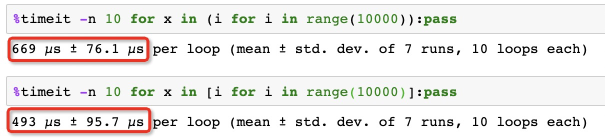
2.generate

先看一组图

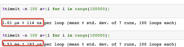
使用()得到的即是一个generator对象，所需要的内存空间与列表的大小无关，所以效率会更高。
but
set 操作

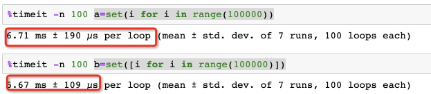
使用set()结果如下
for 操作
使用for()结果如下

大家谨慎使用

3. for循环优化包含多个判断表达式的顺序

对于 and，应该把满足条件少的放在前面，对于 or，把满足条件多的放在前面。
如下：

可见执行条件表达式的顺序，对执行程序还是有一定的影响

4. set与list-交并差

set的union，intersection，difference操作要比list的迭代要快。因此如果涉及到求list交集，并集或者差的问题可以转换为set来操作
如：

5 python垃圾回收机制

import gc
df= pd.DataFrame()
df =...
del def
gc.collect()

6 with open 和open的区别

file = open("test.txt","r")
for line in file.readlines():
    print line
file.close()
和
with open("test.txt","r") as file:
    for line in file.readlines():
       print(line)

等价。
⚠️注意：
• close()是为了释放资源。
• 如果不close()，那就要等到垃圾回收时，自动释放资源。
垃圾回收的时机是不确定的，也无法控制的。如果程序是一个命令，很快就执行完了，那么可能影响不大 （注意：并不是说就保证没问题）。但如果程序是一个服务，或是需要很长时间才能执行完，或者很大并发执 行，就可能导致资源被耗尽，也有可能导致死锁。

file = open("test.txt","r")
for line in file.readlines():
     print (line)
file = open("test.txt","w")
file.write('dsvdfbd')
file = open("test.txt","r")
print('csdfv=\n',file.readline())

如这段代码看不出啥错误～
• 上下文管理器是支持两个方法的对象：enter__和__exit。
with语句实际上是一个非常通用的结构，允许你使用所谓的上下文管理器。
• 方法__enter__不接受任何参数，在进入with语句时被调用，其返回值被赋给关键字as后面的变量。
• 方法__exit__接受三个参数：异常类型、异常对象和异常跟踪。它在离开方法时被调用（通过前述参数将引发的异常提供给它）。如果__exit__返回False，将抑制所有的异常。
• 文件也可用作上下文管理器。它们的方法__enter__返回文件对象本身，而方法__exit__关闭文件

file= open("test.txt","r")
try:
   for line in file.readlines():
       print line
except:
   print "error"
finally:
   file.close()

with语句作用效果相当于上面的try-except-finally

7 context manager

自定义一个上下文管理器类:

class MyResource:
   # __enter__ 返回的对象会被with语句中as后的变量接受
     def __init__(self, x, y):
        self.__x = x
        self.__y = y
   def __enter__(self):
       print('connect to resource')
       return self
   def __exit__(self, exc_type, exc_value, tb):
           print("代码执行到了__exit__......")
        if exc_type == None:
            print('程序没问题')
        else:
            print('程序有问题，如果你能你看懂，问题如下：')
            print('Type: ', exc_type)
            print('Value:', exc_value)
            print('TreacBack:', tb)
        return True
  def sqrt(self):
        print("代码执行到了开更号")
        return math.sqrt(self.__x)

exit: with语句中的代码块执行结束或出错, 会执行_exit__
执行结果如下
connect to resource
代码执行到了开更号
代码执行到了__exit__…
程序有问题，如果你能你看懂，问题如下：

Type:  <class 'ValueError'>
Value: math domain error
TreacBack: <traceback object at 0x10c45ca88>

• 一个简化定义的方法
python提供了一个装饰器contextmanager

from contextlib import contextmanager
class MyResource:
    def query(self):
        print('query data')
@contextmanager
def make_myresource():
    print('start to connect')
    yield MyResource()
    print('end connect')
    pass

被装饰器装饰的函数分为三部分:
with语句中的代码块执行前执行函数中yield之前代码
yield返回的内容复制给as之后的变量
with代码块执行完毕后执行函数中yield之后的代码

8 包相对导入

• from . import spam # 导入当前目录下的spam模块（Python2: 当前目录下的模块, 直接导入即可）
• from .spam import name # 导入当前目录下的spam模块的name属性（Python2: 当前目录下的模块, 直接导入即可，不用加.）
• from … import spam # 导入当前目录的父目录下的spam模块

8.1 包相对导入与普通导入的区别

• from .string import * # 这里导入的string模块为本目录下的(不存在则导入失败) 而不是sys.path路径上的

四 进程

1 joblib’s Parallel

from joblib import Parallel,delayed
def add_labels(filenam,df):
    list_name = list(df['name'])
    if filename in list_name:
 i = list_name.index(filename)
 return df['是否购买][i]
    else:
 return 'Nan'
 
def tmp_func(df1):
    df1['是否购买'] = df1['name'].apply(add_labels, args=(df2,))
    return df
def apply_parallel(df_grouped,func):
    results = Parallel(n_jobs=10)(delayed(func)(group) for name,group in df_grouped)
    return pd.concat(results)
df_grouped = df1.groupby(df1.index)
df1 = apply_parallel(df_grouped,tmp_func)

五 算法相关

1、 KKT条件

考虑带约束的优化问题，可以描述为如下形式

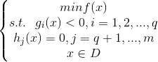
其中f(x)是目标函数，g(x)为不等式约束，h(x)为等式约束。
若f(x)，h(x)，g(x)三个函数都是线性函数，则该优化问题称为线性规划。若任意一个是非线性函数，则称为非线性规划。
若目标函数为二次函数，约束全为线性函数，称为二次规划。

若f(x)为凸函数，g(x)为凸函数，h(x)为线性函数，则该问题称为凸优化。注意这里不等式约束g(x)<=0则要求g(x)为凸函数，若g(x)>=0则要求g(x)为凹函数。

对于同时有多个等式约束和多个不等式约束，构造的拉格朗日函数就是在目标函数后面把这些约束相应的加起来，KKT条件也是如此

参考链接：
[1] https://www.cnblogs.com/liaohuiqiang/p/7805954.html
[2] https://www.jianshu.com/p/df10f536db20?from=timeline&isappinstalled=0
[3] https://www.zhihu.com/question/23311674

1.1 python包sympy求解带约束优化的问题

题目如下：

# 导入sympy包，用于求导，方程组求解等等
from sympy import *

# 设置变量
x1 = symbols("x1")
x2 = symbols("x2")
alpha = symbols("alpha")
beta = symbols("beta")

# 构造拉格朗日等式
L = 10 - x1 * x1 - x2 * x2 + alpha * (x1 * x1 - x2) + beta * (x1 + x2)

# 求导，构造KKT条件
difyL_x1 = diff(L, x1)  # 对变量x1求导
difyL_x2 = diff(L, x2)  # 对变量x2求导
difyL_beta = diff(L, beta)  # 对乘子beta求导
dualCpt = alpha * (x1 * x1 - x2)  # 对偶互补条件

# 求解KKT等式
aa = solve([difyL_x1, difyL_x2, difyL_beta, dualCpt], [x1, x2, alpha, beta])

# 打印结果，还需验证alpha>=0和不等式约束<=0
for i in aa:
    if i[2] >= 0:
        if (i[0] ** 2 - i[1]) <= 0:
            print(i)