机器学习-SVM分类器

import numpy as np
import matplotlib.pyplot as plt
from sklearn.cross_validation import train_test_split
from sklearn.svm import SVC
from sklearn.metrics import classification_report

#加载输入文件中的多变量数据
def load_data(input_file):
    X = []
    y = []
    with open(input_file, 'r') as f:
        for line in f.readlines():
            data = [float(x) for x in line.split(',')]
            X.append(data[:-1])
            y.append(data[-1])
    X = np.array(X)
    y = np.array(y)
    return X, y
#作图函数
def plot_classifier(classifier, X, y, title='Classifier boundaries', annotate=False):
    # define ranges to plot the figure
    x_min, x_max = min(X[:, 0]) - 1.0, max(X[:, 0]) + 1.0
    y_min, y_max = min(X[:, 1]) - 1.0, max(X[:, 1]) + 1.0

    # denotes the step size that will be used in the mesh grid
    step_size = 0.01

    # define the mesh grid
    x_values, y_values = np.meshgrid(np.arange(x_min, x_max, step_size), np.arange(y_min, y_max, step_size))

    # compute the classifier output
    mesh_output = classifier.predict(np.c_[x_values.ravel(), y_values.ravel()])

    # reshape the array
    mesh_output = mesh_output.reshape(x_values.shape)

    # Plot the output using a colored plot
    plt.figure()

    # Set the title
    plt.title(title)

    # choose a color scheme you can find all the options
    # here: http://matplotlib.org/examples/color/colormaps_reference.html
    plt.pcolormesh(x_values, y_values, mesh_output, cmap=plt.cm.gray)

    # Overlay the training points on the plot
    plt.scatter(X[:, 0], X[:, 1], c=y, s=80, edgecolors='black', linewidth=1, cmap=plt.cm.Paired)

    # specify the boundaries of the figure
    plt.xlim(x_values.min(), x_values.max())
    plt.ylim(y_values.min(), y_values.max())

    # specify the ticks on the X and Y axes
    plt.xticks(())
    plt.yticks(())

    if annotate:
        for x, y in zip(X[:, 0], X[:, 1]):
            # Full documentation of the function available here:
            # http://matplotlib.org/api/text_api.html#matplotlib.text.Annotation
            plt.annotate(
                '(' + str(round(x, 1)) + ',' + str(round(y, 1)) + ')',
                xy = (x, y), xytext = (-15, 15),
                textcoords = 'offset points',
                horizontalalignment = 'right',
                verticalalignment = 'bottom',
                bbox = dict(boxstyle = 'round,pad=0.6', fc = 'white', alpha = 0.8),
                arrowprops = dict(arrowstyle = '-', connectionstyle = 'arc3,rad=0'))
#加载输入数据
input_file = 'data_multivar.txt'
X, y = load_data(input_file)
#将数据分类
class_0 = np.array([X[i] for i in range(len(X)) if y[i] == 0])
class_1 = np.array([X[i] for i in range(len(X)) if y[i] == 1])
#绘制数据点
#plt.figure()
#plt.scatter(class_0[:,0], class_0[:,1], facecolor = 'black', edgecolors = 'black', marker = 's')
#plt.scatter(class_1[:,0], class_1[:,1], facecolor = 'None', edgecolors = 'black', marker = 's')
#plt.title('Input Data')

X_train, X_test, y_train, y_test = train_test_split(X, y, test_size=0.25, random_state=5)
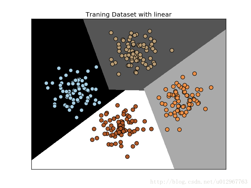
#param = {'kernel':'linear'}     #用线性核函数初始化一个SVM对象
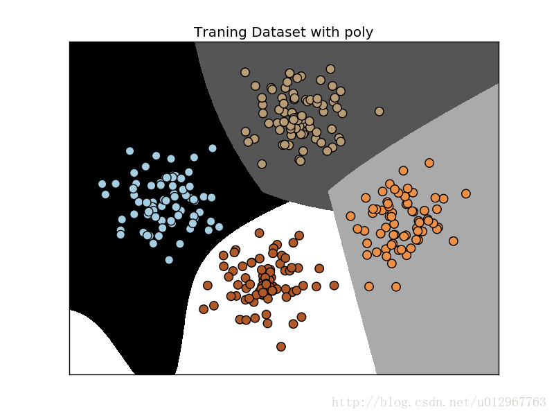
#param = {'kernel':'poly', 'degree':3}#三次多项式方程
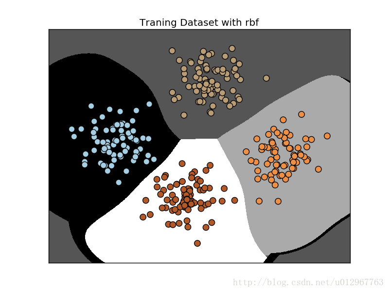
param = {'kernel':'rbf'}        #径向基函数建立非线性分类器
classifier = SVC(**param)
classifier.fit(X_train, y_train)
plot_classifier(classifier, X_train, y_train, 'Traning Dataset')
plt.show()

target_names = ['Class-'+str(int(i))for i in set(y)]
print(classification_report(y_test, classifier.predict(X_test), target_names=target_names))