Bagging – building an ensemble of classifers from bootstrap samples

1. Create a more complex classifcation problem using the Wine dataset

import pandas as pd
df_wine = pd.read_csv('./datasets/wine/wine.data',
                      header=None)
# https://archive.ics.uci.edu/ml/machine-learning-databases/wine/wine.data
df_wine.columns = ['Class label', 'Alcohol', 'Malic acid', 'Ash',
                   'Alcalinity of ash', 'Magnesium', 'Total phenols',
                   'Flavanoids', 'Nonflavanoid phenols', 'Proanthocyanins',
                   'Color intensity', 'Hue', 'OD280/OD315 of diluted wines',
                   'Proline']

# drop 1 class
df_wine = df_wine[df_wine['Class label'] != 1]

y = df_wine['Class label'].values
X = df_wine[['Alcohol', 'Hue']].values

2. Next encode the class labels into binary format and split the dataset into 60 percent training and 40 percent test set, respectively:

from sklearn.preprocessing import LabelEncoder
from sklearn.model_selection import train_test_split
le = LabelEncoder()
y = le.fit_transform(y)

X_train, X_test, y_train, y_test =\
    train_test_split(X, y,
                     test_size=0.40,
                     random_state=1)

3. Use an unpruned decision tree as the base classifer and create an ensemble of 500 decision trees ftted on different bootstrap samples of the training dataset

 

from sklearn.ensemble import BaggingClassifier
tree = DecisionTreeClassifier(criterion='entropy',
                              max_depth=None,
                              random_state=1)

bag = BaggingClassifier(base_estimator=tree,
                        n_estimators=500,
                        max_samples=1.0,
                        max_features=1.0,
                        bootstrap=True,
                        bootstrap_features=False,
                        n_jobs=1,
                        random_state=1)

4. calculate the accuracy score of the prediction on the training and test dataset to compare the performance of the bagging classifer to the performance of a single unpruned decision tree

from sklearn.metrics import accuracy_score
tree = tree.fit(X_train, y_train)
y_train_pred = tree.predict(X_train)
y_test_pred = tree.predict(X_test)

tree_train = accuracy_score(y_train, y_train_pred)
tree_test = accuracy_score(y_test, y_test_pred)
print('Decision tree train/test accuracies %.3f/%.3f'
      % (tree_train, tree_test))

Decision tree train/test accuracies 1.000/0.833

5. The substantially lower test accuracy indicates high variance (overftting) of the model

bag = bag.fit(X_train, y_train)
y_train_pred = bag.predict(X_train)
y_test_pred = bag.predict(X_test)

bag_train = accuracy_score(y_train, y_train_pred)
bag_test = accuracy_score(y_test, y_test_pred)
print('Bagging train/test accuracies %.3f/%.3f'
      % (bag_train, bag_test))

Bagging train/test accuracies 1.000/0.896

6.  compare the decision regions between the decision tree and bagging classifer

x_min = X_train[:, 0].min() - 1
x_max = X_train[:, 0].max() + 1
y_min = X_train[:, 1].min() - 1
y_max = X_train[:, 1].max() + 1

xx, yy = np.meshgrid(np.arange(x_min, x_max, 0.1),
                     np.arange(y_min, y_max, 0.1))

f, axarr = plt.subplots(nrows=1, ncols=2,
                        sharex='col',
                        sharey='row',
                        figsize=(8, 3))


for idx, clf, tt in zip([0, 1],
                        [tree, bag],
                        ['Decision Tree', 'Bagging']):
    clf.fit(X_train, y_train)

    Z = clf.predict(np.c_[xx.ravel(), yy.ravel()])
    Z = Z.reshape(xx.shape)

    axarr[idx].contourf(xx, yy, Z, alpha=0.3)
    axarr[idx].scatter(X_train[y_train == 0, 0],
                       X_train[y_train == 0, 1],
                       c='blue', marker='^')

    axarr[idx].scatter(X_train[y_train == 1, 0],
                       X_train[y_train == 1, 1],
                       c='red', marker='o')

    axarr[idx].set_title(tt)

axarr[0].set_ylabel('Alcohol', fontsize=12)
plt.text(10.2, -1.2,
         s='Hue',
         ha='center', va='center', fontsize=12)
plt.show()

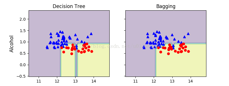
7. Results:

The piece-wise linear decision boundary of the three-node deep decision tree looks smoother in the bagging ensemble