FTRL(Follow The Regularized Leader)学习总结

最新推荐文章于 2023-05-08 02:04:24 发布

AcceptedLin

最新推荐文章于 2023-05-08 02:04:24 发布

阅读量1.1k

点赞数

分类专栏：机器学习 Python

原文链接：https://www.cnblogs.com/arachis/p/FTRL.html

版权

机器学习同时被 2 个专栏收录

135 篇文章

订阅专栏

Python

125 篇文章

订阅专栏

FTRL(Follow The Regularized Leader)学习总结

摘要：

　　1.算法概述

　　2.算法要点与推导

　　3.算法特性及优缺点

　　4.注意事项

　　5.实现和具体例子

　　6.适用场合

内容：

　1.算法概述

　　FTRL是一种适用于处理超大规模数据的,含大量稀疏特征的在线学习的常见优化算法，方便实用，而且效果很好，常用于更新在线的CTR预估模型；

　　FTRL算法兼顾了FOBOS和RDA两种算法的优势，既能同FOBOS保证比较高的精度，又能在损失一定精度的情况下产生更好的稀疏性。

　　FTRL在处理带非光滑正则项（如L1正则）的凸优化问题上表现非常出色，不仅可以通过L1正则控制模型的稀疏度，而且收敛速度快；

　　参考：[笔记]FTRL与Online Optimization

　2.算法要点与推导

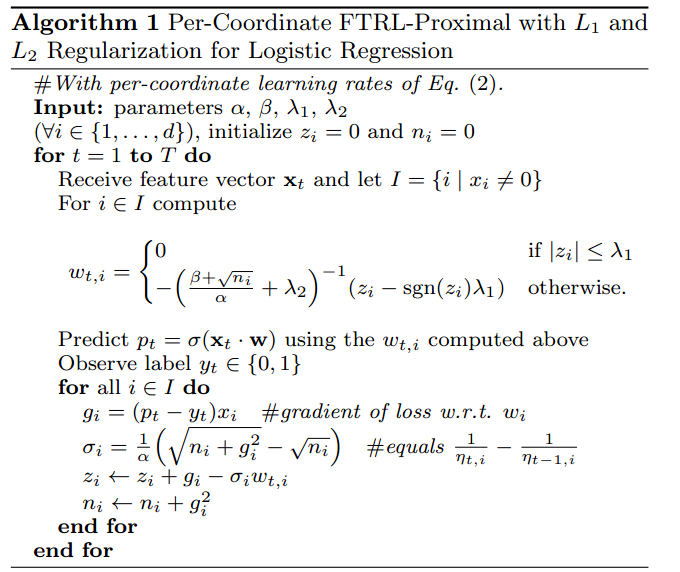
　3.算法特性及优缺点

　　FTRL-Proximal工程实现上的tricks：

　　1.saving memory

　　　　方案1）Poisson Inclusion：对某一维度特征所来的训练样本，以p的概率接受并更新模型。
　　　　方案2）Bloom Filter Inclusion：用bloom filter从概率上做某一特征出现k次才更新。

　　2.浮点数重新编码

　　　　1）特征权重不需要用32bit或64bit的浮点数存储，存储浪费空间
　　　　2）16bit encoding，但是要注意处理rounding技术对regret带来的影响(注：python可以尝试用numpy.float16格式)
　　3.训练若干相似model
　　　　1）对同一份训练数据序列，同时训练多个相似的model
　　　　2）这些model有各自独享的一些feature，也有一些共享的feature
　　　　3）出发点：有的特征维度可以是各个模型独享的，而有的各个模型共享的特征，可以用同样的数据训练。
　　4.Single Value Structure
　　　　1）多个model公用一个feature存储（例如放到cbase或redis中），各个model都更新这个共有的feature结构
　　　　2）对于某一个model，对于他所训练的特征向量的某一维，直接计算一个迭代结果并与旧值做一个平均
　　5.使用正负样本的数目来计算梯度的和（所有的model具有同样的N和P）

　　6.subsampling Training Data
　　　1）在实际中，CTR远小于50%，所以正样本更加有价值。通过对训练数据集进行subsampling，可以大大减小训练数据集的大小
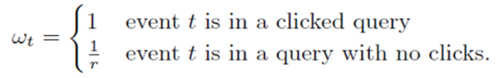
　　　2）正样本全部采（至少有一个广告被点击的query数据），负样本使用一个比例r采样（完全没有广告被点击的query数据）。但是直接在这种采样上进行训练，会导致比较大的biased prediction
　　 3）解决办法：训练的时候，对样本再乘一个权重。权重直接乘到loss上面，从而梯度也会乘以这个权重。

算法特点：

在线学习，实时性高；
可以处理大规模稀疏数据；
有大规模模型参数训练能力；
根据不同的特征特征学习率。

实现和具体例子：

FTRL处理“Springleaf Marketing Response”数据

Spark Streaming on Angel FTRL

适用场合：点击率模型

代码：

from datetime import datetime
from csv import DictReader
from math import exp, log, sqrt
from random import random
import pickle

# TL; DR, the main training process starts on line: 250,
# you may want to start reading the code from there


##############################################################################
# parameters #################################################################
##############################################################################

# A, paths
train='../input/train.csv'
test='../input/test.csv'#'vali_100.tsv'
submission = 'ftrl1sub.csv'  # path of to be outputted submission file

# B, model
alpha = .005  # learning rate
beta = 1.   # smoothing parameter for adaptive learning rate
L1 = 0.     # L1 regularization, larger value means more regularized
L2 = 1.     # L2 regularization, larger value means more regularized

# C, feature/hash trick
D = 2 ** 24             # number of weights to use
interaction = False     # whether to enable poly2 feature interactions

# D, training/validation
epoch = 1       # learn training data for N passes
holdafter = 9   # data after date N (exclusive) are used as validation
holdout = None  # use every N training instance for holdout validation


##############################################################################
# class, function, generator definitions #####################################
##############################################################################

class ftrl_proximal(object):
    ''' Our main algorithm: Follow the regularized leader - proximal

        In short,
        this is an adaptive-learning-rate sparse logistic-regression with
        efficient L1-L2-regularization

        Reference:
        http://www.eecs.tufts.edu/~dsculley/papers/ad-click-prediction.pdf
    '''

    def __init__(self, alpha, beta, L1, L2, D, interaction):
        # parameters
        self.alpha = alpha
        self.beta = beta
        self.L1 = L1
        self.L2 = L2

        # feature related parameters
        self.D = D
        self.interaction = interaction

        # model
        # n: squared sum of past gradients
        # z: weights
        # w: lazy weights
        self.n = [0.] * D
        self.z = [random() for k in range(D)]#[0.] * D
        self.w = {}

    def _indices(self, x):
        ''' A helper generator that yields the indices in x

            The purpose of this generator is to make the following
            code a bit cleaner when doing feature interaction.
        '''

        # first yield index of the bias term
        yield 0

        # then yield the normal indices
        for index in x:
            yield index

        # now yield interactions (if applicable)
        if self.interaction:
            D = self.D
            L = len(x)

            x = sorted(x)
            for i in xrange(L):
                for j in xrange(i+1, L):
                    # one-hot encode interactions with hash trick
                    yield abs(hash(str(x[i]) + '_' + str(x[j]))) % D

    def predict(self, x):
        ''' Get probability estimation on x

            INPUT:
                x: features

            OUTPUT:
                probability of p(y = 1 | x; w)
        '''

        # parameters
        alpha = self.alpha
        beta = self.beta
        L1 = self.L1
        L2 = self.L2

        # model
        n = self.n
        z = self.z
        w = {}

        # wTx is the inner product of w and x
        wTx = 0.
        for i in self._indices(x):
            sign = -1. if z[i] < 0 else 1.  # get sign of z[i]

            # build w on the fly using z and n, hence the name - lazy weights
            # we are doing this at prediction instead of update time is because
            # this allows us for not storing the complete w
            if sign * z[i] <= L1:
                # w[i] vanishes due to L1 regularization
                w[i] = 0.
            else:
                # apply prediction time L1, L2 regularization to z and get w
                w[i] = (sign * L1 - z[i]) / ((beta + sqrt(n[i])) / alpha + L2)

            wTx += w[i]

        # cache the current w for update stage
        self.w = w

        # bounded sigmoid function, this is the probability estimation
        return 1. / (1. + exp(-max(min(wTx, 35.), -35.)))

    def update(self, x, p, y):
        ''' Update model using x, p, y

            INPUT:
                x: feature, a list of indices
                p: click probability prediction of our model
                y: answer

            MODIFIES:
                self.n: increase by squared gradient
                self.z: weights
        '''

        # parameter
        alpha = self.alpha

        # model
        n = self.n
        z = self.z
        w = self.w

        # gradient under logloss
        g = p - y

        # update z and n
        for i in self._indices(x):
            sigma = (sqrt(n[i] + g * g) - sqrt(n[i])) / alpha
            z[i] += g - sigma * w[i]
            n[i] += g * g


def logloss(p, y):
    ''' FUNCTION: Bounded logloss

        INPUT:
            p: our prediction
            y: real answer

        OUTPUT:
            logarithmic loss of p given y
    '''

    p = max(min(p, 1. - 10e-15), 10e-15)
    return -log(p) if y == 1. else -log(1. - p)


def data(path, D):
    ''' GENERATOR: Apply hash-trick to the original csv row
                   and for simplicity, we one-hot-encode everything

        INPUT:
            path: path to training or testing file
            D: the max index that we can hash to

        YIELDS:
            ID: id of the instance, mainly useless
            x: a list of hashed and one-hot-encoded 'indices'
               we only need the index since all values are either 0 or 1
            y: y = 1 if we have a click, else we have y = 0
    '''

    for t, row in enumerate(DictReader(open(path), delimiter=',')):
        # process id
        #print row
        
        try:
            ID=row['ID']
            del row['ID']
        except:
            pass
        # process clicks
        y = 0.
        target='target'#'IsClick' 
        if target in row:
            if row[target] == '1':
                y = 1.
            del row[target]

        # extract date

        # turn hour really into hour, it was originally YYMMDDHH

        # build x
        x = []
        for key in row:
            value = row[key]

            # one-hot encode everything with hash trick
            index = abs(hash(key + '_' + value)) % D
            x.append(index)

        yield ID,  x, y


##############################################################################
# start training #############################################################
##############################################################################

start = datetime.now()

# initialize ourselves a learner
learner = ftrl_proximal(alpha, beta, L1, L2, D, interaction)

# start training
for e in range(epoch):
    loss = 0.
    count = 0
    for t,  x, y in data(train, D):  # data is a generator

        p = learner.predict(x)
        loss += logloss(p, y)
        learner.update(x, p, y)
        count+=1
        if count%1000==0:
            #print count,loss/count
            print('%s\tencountered: %d\tcurrent logloss: %f' % (
                datetime.now(), count, loss/count))
        if count>10000: # comment this out when you run it locally.
            break


count=0
loss=0
#import pickle
#pickle.dump(learner,open('ftrl3.p','w'))
print ('write result')
##############################################################################
# start testing, and build Kaggle's submission file ##########################
##############################################################################
with open(submission, 'w') as outfile:
    outfile.write('ID,target\n')
    for  ID, x, y in data(test, D):
        count+=1
        p = learner.predict(x)
        loss += logloss(p, y)

        outfile.write('%s,%s\n' % (ID, str(p)))
        if count%1000==0:
            #print count,loss/count
            print('%s\tencountered: %d\tcurrent logloss: %f' % (
                datetime.now(), count, loss/count))