《Processing SPARQL queries over distributed RDF graphs》——读书笔记

这次读论文给了我惨痛的教训，不做笔记是不行的，越长的论文越应该做笔记！不可怠惰！

Abstract

propose techniques for processing SPARQL queries over a large RDF graph in a distributed environment.
“partial evaluation and assembly” framework.
partial evaluation——在每个子图中找到部分匹配的答案。
assembly——centralized and distributed.

1 Introduction

语义网数据模型，(Resource Description Framework, RDF).
数据大量增长，与之相应地，计算和存储需求增加，超出单个机器的能力。
关于distributed evaluation of SPARQL queries over large RDF datasets 大体上有三类方法。
1) Cloud-based approaches maintain a large RDF graph using existing cloud computing platforms, such as Hadoop or Cassandra, and employ triple pattern-based join processing most commonly using MapReduce.
2) Partition-based approaches divide the RDF graph Ginto a set of subgraphs (fragments) and decompose the SPARQL query Q into subqueries. These subqueries are then executed over the partitioned data using techniques similar to relational distributed databases.
3) Federated approaches. Federated SPARQL processing systems evaluate queries over multiple SPARQL endpoints. These systems typically target LOD and follow a query processing over data integration approach.

本文的策略是划分图但不拆解查询。RDF图被拆解成顶点不相交的段。每个站点都接受完整的查询，并行计算。该方法是首次应用于该方向，中间结果少。

基于Partial Evaluation的分布式数据管理中，每个机器将存储在自身的数据视为已知的部分s，而存储在其他机器上的数据视为未知的部分d。然后，每个机器利用已知部分对查询求出部分解。最后，这些局部匹配被收集起来并通过连接操作拼成最终解。—— 来自彭鹏的知乎回答
Within the context of graph processing, the technique has been used to evaluate reachability queries and graph simulation over graphs.
但是 SPARQL is based on graph homomorphism. SPARQL query semantics is different than these (上文中的可达性查询和图同构).

Some SPARQL query matches are contained within a fragment, which we call inner matches.
Subgraph matches that cross multiple fragments are called crossing matches.
该框架主要需要解决两个问题：一是计算在每个站点中查询Q的部分评价结果。二是组合这些部分匹配的结果得到答案。
方法的优点有两方面：
一是不依赖于特定的图的划分策略。
二是保证中间结果的点和边比别的方法少。

2 Related work

2.1 Distributed SPARQL query processing

2.1.1 Cloud-based approaches

HDFS-based approaches

他们将RDF三元组以flat files的格式存储到HDFS中。进行SPARQL查询的时候，先扫一遍HDFS文件，然后使用MapReduce进行连接。这些方法的不同主要在于如何将RDF三元组存储到HDFS文件中。
SHARD 直接存到一个文件中，每行表示一个特定主体的所有三元组。
HadoopRDF and PredicateJoin 基于谓词划分三元组，每个划分存到一个文件中。
EAGRE 将具有相似属性的主体合成一个实体类，然后构造一个仅包含实体类及其之间连接的压缩RDF图。使用METIS算法划分图。

No HDFS-based approaches

Besides the HDFS-based approaches, there are also some works that use other NoSQL distributed data stores to manage RDF datasets.
JenaHBase and $H_2$RDF 利用主体、客体、谓词的排列建立索引并存储到HBase中。
Trinity.RDF uses the distributed memory-cloud graph system Trinity to index and store the RDF graph.

基于云的方法得益于云平台的高可扩展性和容错能力，但是因MapReduce难以适配到图计算中导致性能较低。

2.1.2 Partition-based approaches

如上文所述，就是把图和查询都分解。但因分解方法的不同，查询的处理方法也不同。
GraphPartition 通过边界点的N条邻居来得到每个段。
WARP uses some frequent structures in workload to further extend the results of GraphPartition.
Partout…
TriAD METIS 划分RDF图。并且结果的块数比site数要多。

但是有一些情况是需要根据特定的需求来划分数据的。这些根据方法去划分的方法不够灵活。

2.1.3 Federated SPARQL query systems

Federated queries run SPARQL queries over multiple SPARQL endpoints. A typical example is linked data, where different RDF repositories are interconnected, providing a virtually integrated distributed database. (与文章不相关，我不做笔记了)

2.2 Partial evaluation

与第一章类似，介绍了部分评价的应用，如在分布式XML中进行XPath查询，图的同构查询等等。详细介绍了图同构（多项式时间可解）与图同态（完全NP问题）的区别。

3 Background and framework

Definition 1
(RDF graph) An RDF graph is denoted as $G=\{V,E, \Sigma\}$, where V is a set of vertices that correspond to all subjects and objects in RDF data; $E \subseteq V \times V$ is a multiset of directed edges that correspond to all triples in RDF data; $\Sigma$ is a set of edge labels. For each edge $e\in E$, its edge label is its corresponding property.

同样的，SPARQL查询同样可以表示为图。我们首次关注basic graph pattern (BGP) qurries。在第六章有详细的讨论。
Definition 2
(SPARQL BGP query) A SPARQL BGP query is denoted as $Q=\{V^Q,E^Q, \Sigma^Q\}$, where $V^Q\subseteq V\cup V_{Var}$ is a set of vertices, where V denotes all vertices in RDF graph G and $V_{Var}$ is a set of variables; $E^Q \subseteq V^Q \times V^Q$ is a multiset of edges in Q; each edge e in $E^Q$ either has an edge label in $\Sigma$ or the edge label is a variable.
Definition 3
(SPARQL match) Consider an RDF graph G and a connected query graph Q that has n vertices $\{v_1,..,v_n \}$. A subgraph M with m vertices $\{u_1,..,u_m \}$(in G) is said to be a match of Q if and only if there exists a functionf from $\{v_1,...,v_n \}$to $\{u_1,..,u_m \}(n\ge m)$, where the following condition hold:

1. if $v_i$ is not a variable, $f(v_i)$ and $v_i$ have the same URI or literal value $(1\le i\le n)$;
2. if $v_i$ is a variable, there is no constraint over $f(v_i)$ except that $f(v_i)\in \{u_1,..,u_m \}$;
3. if there exists an edge $\overrightarrow{v_iv_j}$ in Q, there also exists an edge $\overrightarrow{f{(v_i)}f{(v_j)}}$ in G. Let $L(\overrightarrow{v_iv_j})$ denote a multi-set of labels between $v_i$ and $v_j$ in Q; and $L(\overrightarrow{f{(v_i)}f{(v_j)}}$ denote a multi-set of labels between $f{(v_i)}$ and $f{(v_j)}$ in G. There must exist an injective function from edge labels in $L(\overrightarrow{v_iv_j})$ to edge labels in $L(\overrightarrow{f{(v_i)}f{(v_j)}}$. Note that a variable edge label in $L(\overrightarrow{v_iv_j})$ can match any edge label in $L(\overrightarrow{f{(v_i)}f{(v_j)}}$.

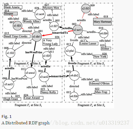
图被划分为不同的段，不同的分布式RDF系统使用不同的划分算法，但是我们的方法对划分算法不敏感。

Definition 4
(Distributed RDF graph) A distributed RDF graph $G=\{V,E,\Sigma \}$ consists of a set of fragments $\mathcal {F} = \{F_1,F_2,\ldots ,F_k\}$ where each $F_i$ is specified by $(V_i \cup V_i^e, E_i \cup E_i^c, \varSigma _i)(i=1,...,k)$ such that

1. $\{V_1,\ldots ,V_k\}$ is a partitioning of V, i.e., $V_i \cap V_j = \emptyset ,1 \le i,j \le k,i \ne j$ and $\bigcup \nolimits _{i = 1,\ldots ,k} {V_i = V}$
2. $E_i \subseteq V_i \times V_i, i=1,...,k$;
3. $E_i^c$ is a set of crossing edges between $F_i$ and other fragments, i.e., （交叉边定义）
4. a vertex $u^{'}\in V_i^e$ if and only if vertex $u^{'}$ resides in another fragment $F_j$ and $u^{'}$ is an endpoint of a crossing edge between fragment $F_i and F_j(F_i\ne F_j)$,i.e., $$\begin{aligned} V_i^e&= \left( \bigcup \nolimits _{1 \le j \le k \wedge j \ne i} \{ {u^\prime } |\overrightarrow{uu^\prime }\,\in E_i ^c \wedge u \in F_i \} \right) \bigcup \\&\quad \quad \left( \bigcup \nolimits _{1 \le j \le k \wedge j \ne i} {\{ {u^\prime } |\overrightarrow{u^\prime u} \in E_i ^c \wedge u \in F_i \} }\right) \end{aligned}$$ ;（外部点集合）
5. Vertices in $V_i^e$ are called extended vertices of $F_i$, and all vertices in $V_i$ are called internal vertices of $F_i$;(内部点和外部点)
6. $\varSigma _i$ is a set of edge labels in $F_i$

Definition 5
(Problem statement) Let G be a distributed RDF graph that consists of a set of fragments $\mathcal {F} = \{F_{1}, \ldots , F_{k}\}$ and let $\mathcal {S} = \{S_{1}, \ldots , S_{k}\}$ be a set of computing nodes such that $F_i$ is located at $S_i$. Given a SPARQL query graph Q, our goal is to find all SPARQL matches of Q in G.

段内能匹配的问题，不再考虑，主要研究跨段匹配问题。
There are three steps in our method.
Step 1 (Initialization): A SPARQL query Q is input and sent to each site in S.
Step 2 (Partial Evaluation): Each site Si finds local partial matches of Q over fragment Fi. This step is executed in parallel at each site (Sect. 4).
Step 3 (Assembly): Finally, we assemble all local partial matches to compute complete crossing matches. The system can use the centralized (Sect. 5.2) or the distributed assembly approach (Sect. 5.3) to find crossing matches.

4 Partial evaluation

4.1 Local partial match: definition

Definition 6
(Local partial match) Given a SPARQL query graph Q with n vertices$\{v_1,...,v_n \}$ and a connected subgraph PM with m vertices$\{u_1,...,u_m \}(m\le n)$in a fragment $F_k$, PM is a local partial match in fragment $F_k$ if and only if there exists a function $f: \{v_1,...,v_n\} \rightarrow \{u_1,...,u_m \}\cup \{NULL\}$, where the following conditions hold:

1. If $v_i$ is not a variable, $f(v_i)$ and $v_i$ have the same URI or literal or $f(v_i)=NULL$
2. If $v_i$ is a variable, $f(v_i)\in \{u_1,...,u_m \}$or $f(v_i)=NULL$
3. If there exists an edge $\overrightarrow{v_iv_j}$in $Q(1\le i\ne j\le n),$ then PM must meet one of the following five conditions:(1) there also exists an edge $\overrightarrow{f{(v_i)}f{(v_j)}}$in PM with property p, and p is the same to the property of $\overrightarrow{v_iv_j}$; (2) there also exists an edge $\overrightarrow{f{(v_i)}f{(v_j)}}$ in PM with property p, and the property of $\overrightarrow{v_iv_j}$ is a variable; (3) there does not exist an edge $\overrightarrow{f{(v_i)}f{(v_j)}}$, but $f(v_i)$ and $f(v_j)$ are both in $V_k^e$; (4) $f(v_i)=NULL$; (4) $f(v_j)=NULL$;
4. PM contains at least one crossing edge, which guarantees that an empty match does not qualify.
5. If $f(v_i) \in V_k$ (i.e., $f(v_i)$ is an internal vertex in $F_k$) and $\exists \overrightarrow{v_i v_j} \in Q$(or $\overrightarrow{v_j v_i} \in Q$), there must exist $f(v_j) \ne NULL$ and $\exists \overrightarrow{f(v_i)f(v_j)} \in PM$ (or $\exists \overrightarrow{f(v_j)f(v_i)} \in PM$). Furthermore, if $\overrightarrow{v_i v_j}$(or $\overrightarrow{v_j v_i}$) has a property p, $\overrightarrow{f(v_i)f(v_j)}$ (or $\overrightarrow{f(v_j)f(v_i)}$) has the dame property p.
6. Any two vertices $v_i$ and $v_j$ (in query Q), where $f(v_i)$ and $f(v_j)$ are both internal vertices in PM, are weakly connected in Q.
   Vector $[f(v_1),...,f(v_n)]$ is a serialization of a local partial match.

The basic intuition of Condition 5 is that if vertex vivi (in query Q) is matched to an internal vertex, all of vivi’s neighbors should be matched in this local partial match as well.

Definition 7
Two vertices are weakly connected in a directed graph if and only if there exists a connected path between the two vertices when all directed edges are replaced with undirected edges. The path is called a weakly connected path between the two vertices.

The correctness of our method is stated in the following propositions.

1.The overlapping part between any crossing match M and internal vertices of fragment FiFi (i=1,…,ki=1,…,k) must be a local partial match (see Proposition 1).
2.Missing any local partial match may lead to result dismissal. Thus, the algorithm should find all local partial matches in each fragment (see Proposition 2).
3.It is impossible to find two local partial matches M and M′M′ in fragment F, where M′M′ is a subgraph of M, i.e., each local partial match is maximal (see Proposition 4).

Proposition 1
Given any crossing match M of SPARQL query Q in an RDF graph G, if M overlaps with some fragment $F_i$, let $(M\cup F_i)$ denote the overlapping part between M and fragment $F_i$. Assume that $(M\cup F_i)$ consists of several weakly connected components, denoted as $(M\cup F_i)=\{PM_1,...,PM_n\}$. Each weakly connected component $PM_a(1\le a\le n)$ in $(M\cup F_i)$ must be a local partial match in fragment $F_i$.(证明有定义六中的六个条件即可。)
Proposition 2
The partial evaluation and assembly algorithm does not miss any crossing matches in the answer set if and only if all local partial matches in each fragment are found in the partial evaluation stage.（反证法分别证明充分性和必要性。）保证了没有local partial matches丢失。
Proposition 3
Given the same underlying partitioning over RDF graph G, the number of involved vertices and edges in the intermediate results (in our approach) is not larger than that in any other partition-based solution.（反证法证明本方法的每个点和每个边其他方法都需要有，否则结果不全）保证了中间结果包含的点和边最少。
Proposition 4
Given a query graph Q and an RDF graph G, if $PM_i$ is a local partial match under function f in fragment $F_i$, there exists no local partial match $PM^{'}_i$ under function $f^{'}$ in $F_i$,where $f\subset f^{'}$

Any PMiPMi cannot be enlarged by introducing more vertices or edges to become a larger local partial match.

4.2 Computing local partial matches

部分评价的目标就是在$F_i$中找到Q的点对应的点，建立起一个映射f。f可以表示为一系列的点对。算法如下：


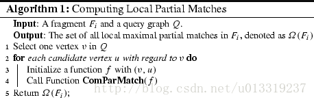
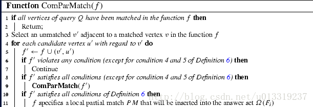
修改原来用作子图匹配的gStore，用来计算local partial matches.
状态转移算法

5 Assembly

找到每个fragment部分评价的结果后，就是组装这些结果。有两种策略：
centralized——所有部分评价的匹配对送至一个站点组装。
distributed (or parallel)——部分匹配对在多个站点同时匹配。

5.1 Join-based assembly

Definition 8(可连接的条件)
(Joinable) Given a query graph Q and two fragments $F_i$ and $F_j (i\ne j)$, let $PM_i$ and $PM_j$ be the corresponding local partial matches over fragments $F_i$ and $F_j$ under functions $f_i$ and $f_j$. $PM_i$ and $PM_j$ are joinable if and only if following conditions hold:

1. There exist no vertices u and $u^{'}$ in $PM_i$ and $PM_j$, respectively, such that $f_i^{-1}(u)=f_j^{-1}(u^{'})$(没有重合点)
2. There exists at least on crossing edge $\vec{uu^{'}}$ such that u is an internal vertex and $u^{'}$ is an extended vertex in $F_i$, while u is an extended vertex and $u^{'}$ is an internal vertex in $F_j$. Furthermore, $f_i^{-1}(u)=f_j^{-1}(u)$ and $f_i^{-1}(u^{'})=f_j^{-1}(u^{'})$(至少有一个公共边)
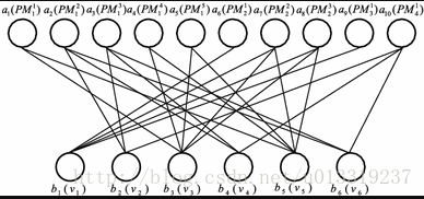
   Definition 9
   (Join result) Given a query graph Q and two fragments $F_i$ and $F_j (i\ne j)$, let $PM_i$ and $PM_j$ be two joinable local partial matches of Q over fragments $F_i$ and $F_j$ under functions $f_i$ and $f_j$, respectively. The join of $PM_i$ and $PM_j$ is defined under a new function f (donoted as $PM=PM_i\bowtie_f PM_j$), which is defined as follows for any vertex v in Q:
3. if $f_i(v)\ne NULL \wedge f_j(v)=NULL,f(v)\leftarrow f_i(v)$;
4. if $f_i(v)=NULL \wedge f_j(v)\ne NULL,f(v)\leftarrow f_j(v)$;
5. if $f_i(v)\ne NULL \wedge f_j(v)\ne NULL,f(v)\leftarrow f_i(v)(In this case, f_i(v)=f_j(v))$;
6. if $f_i(v)=NULL \wedge f_j(v)= NULL,f(v)\leftarrow NULL$;
   (这个连接没什么好解释的，具体参考图3就好了。就是把两个f揉到一个里面)

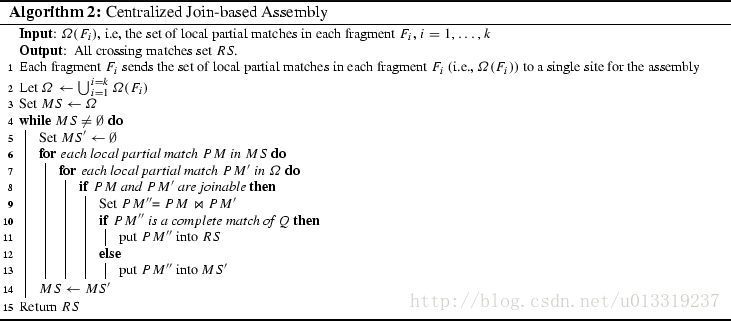
5.2 Centralized assembly

集中组装，所有的PM都被送至一个最终组装点。提出了一个迭代连接算法（算法2）。

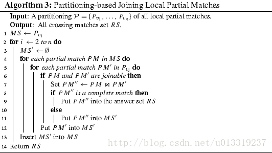
5.2.1 Partitioning-based join processing

为了降低连接空间。
Theorem 1
Given two local partial matches $PM_i$ and $PM_j$ from fragments $F_i$ and $F_j with functions$f_i$and$f_j$, respectively, if there exists a query vertex v where both$f_i(v)$and$f_j(v)$are internal vertices of fragments$F_i$and$F_j$, respectively,$PM_i$and$PM_j$ are not joinable.
(如果query中的某个点对应到两个PM中都是内部点，那这两个PM肯定不能相连)
Definition 10
(Local partial match partitioning). Consider a SPARQL query Q with n vertices ${v_i,...,v_n}$. Let $\Omega$ denote all local partial matches. $P={P_{v1},...,P_{vn}}$ is a partitioning of $\Omega$ if and only if the following conditions hold.

1. Each partition P_{vi}(i=1,…,n) consists of a set of local partial matches, each of which has an internal vertex that matches $v_i$.
2. $P_{vi}\cap P_{vj}=\varnothing$, where $1\le i\ne j \le n$
3. $P_{v1}\cup ...\cup P_{vn}= \Omega$
   定义了PM的划分方式，只有在不同块的PM才可能join。Algorithm 3 shows how to perform partitioning-based join of local partial matches.
   

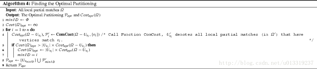
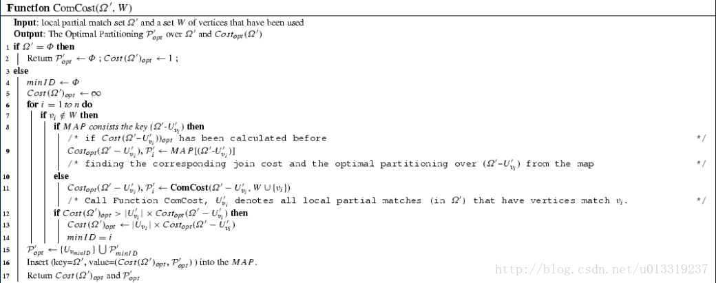
5.2.2 Finding the optimal partitioning

为找到最佳的划分方式。先定义划分花费用来衡量划分方案。
Definition 11
(Join cost). Given a query graph Q with n vertices $v_1,...,v_n$ and a partitioning $P={P_{v1},...,P_{vn}}$ over all local partial matches $\Omega$, the join cost is

$$Cost(\Omega)=O\left(\prod_{i=1}^{i=n}(|P_{vi}|+1) \right)$$
where $|P_{vi}|$ is the number of local partial matches in $P_{vi}$and 1 is introduced to avoid the ‘0’ element in the product.
假设每个来自不同分区的LPM都是可连接的，来计算最差情况下的花费。

Definition 12
(Optimal partitioning). Given a partitioning P over all local partial matches $\Omega$, P is the optimal partitioning if and only if there exists no another partitioning that has smaller join cost.
(定义了最优的划分方式)
Theorem 2
Finding the optimal partitioning is NP-complete problem.

Proof
We can reduce a 0-1 integer planning problem to finding the optimal partitioning.

We formulate the 0-1 integer planning problem as follows:

$$\min \prod \limits _{i = 0}^{i = n} \left( \sum \limits _j {x_{ji} } + 1\right) \\ \quad \hbox {st.}\forall j,\sum \limits _i {x_{ji} } = 1$$
The equivalence between the 0-1 integer planning and finding the optimal partitioning are straightforward. The former is a classical NP-complete problem. Thus, the theorem holds.
Theorem 3
Given a query graph Q with n vertices $v_1,..,v_n$ and a set of all local partial matches $\Omega$, let $U_{vi}$(i=1,…,n) be all local partial matches (in $\Omega$) that have internal vertices matching $v_i$. For the optimal partitioning $P_{opt}={P_{v1},...,P_{vn}}$ where $P_{vn}$ has the largest size (i.e., the number of local partial matches in $P_{vn}$ is maximum) in $P_{opt}, P_{vn}=U_{vn}$
问题在于如何利用定理3找到一个最优的序列。
$$\begin{aligned} Cost(\varOmega )_{opt}= & {} |P_{v_{k_1 } } | \times Cost(\varOmega _{\overline{v_{k_1 } } } )_{opt} \nonumber \\= & {} |U_{v_{k_1 } } | \times Cost(\varOmega _{\overline{v_{k_1 } } } )_{opt} \end{aligned}$$
但是我们不知道哪一个是 $v_{k1}$引入以下结构：
$$\begin{aligned} Cost(\varOmega )_{opt}= & {} MIN_{1 \le i \le n} (|P_{v_i } | \times Cost(\varOmega _{\overline{v_i } } )_{opt} ) \nonumber \\= & {} MIN_{1 \le i \le n} (|U_{v_i } | \times Cost(\varOmega _{\overline{v_i } } )_{opt} ) \end{aligned}$$
上式可以利用中间结果，再优化：
$$\begin{aligned} Cost(\varOmega )_{opt}= & {} MIN_{1 \le i \le n;1 \le j \le n;i \ne j} (|P_{v_i } | \times |P_{v_j } | \nonumber \\&\times Cost(\varOmega _{\overline{v_i v_j } } )_{opt} ) \nonumber \\= & {} MIN_{1 \le i \le n;1 \le j \le n;i \ne j} (|U_{v_i } | \times |U_{v_j }^{\prime }| \nonumber \\&\times Cost(\varOmega _{\overline{v_i v_j } } )_{opt} ) \end{aligned}$$

5.2.3 Join order

如果最优的划分确定了，则连接顺序也确定了。If the optimal partitioning is $\mathcal {P}_{opt}=\{P_{v_{k_1}},\ldots ,P_{v_{k_n}}\}$ and $|P_{v_{k_1}}| \ge |P_{v_{k_2}}| \ge \ldots \ge |P_{v_{k_n}}|$, then the join order must be $P_{v_{k_1}} \bowtie P_{v_{k_2}} \bowtie \ldots \bowtie P_{v_{k_n}}$. 原因如下：
First, changing the join order may not prune any intermediate results.
Second, in some special cases, the join order may have an effect on the performance.

5.3 Distributed assembly

We adopt Bulk Synchronous Parallel (BSP) model to design a synchronous algorithm for distributed assembly. A BSP computation proceeds in a series of global supersteps, each of which consists of three components: local computation, communication and barrier synchronization.

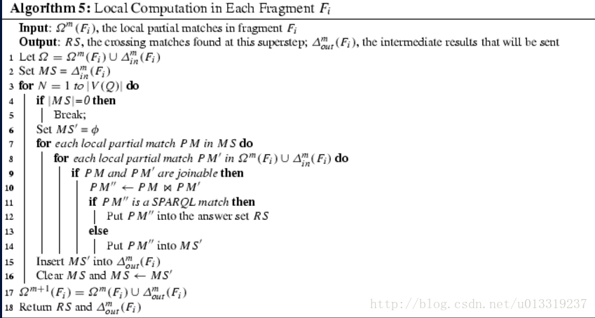
5.3.1 Local computation

Consider the mth superstep. For each fragment $F_i$, let $\varDelta _{in}^{m}(F_i)$ denote all received intermediate results in the mth superstep and $\varOmega ^{m}(F_i)$ denote all local partial matches and the intermediate results generated in the first (m−1) supersteps.

5.3.2 Communication

为了防止两个fragment互发PM导致重复结果，需根据fragment中的PM数量进行排序。
Definition 13
Given any two fragments $F_i and F_j$, $F_i \prec F_j$ if and only if $|\Omega(F_i)|\le|\Omega(F_j)|(1\le i,j\le n)$.
采用分治法。
Assume that PM is generated by joining intermediate results from m different fragments $F_{i1},…,F_{im}$ , where $F_{i1}≺F_{i2}≺…≺F_{im}$. We send PM to another fragment $F_j$ if and only if two conditions hold: (1) $F_j>F_{im}$ ; and (2) $F_j$ shares common crossing edges with at least one fragment of $F_{i1} ,..., F_{im}$.

5.3.3 Barrier synchronization

第m步的沟通必须在第m+1步之前完成。
初始状态的时候，只有本地的匹配结果，但不可能连接，所以不需要计算，直接进入communication阶段。直接发送$\Omega_{F_i}$到别的fragment。

5.3.4 System termination condition

BSP算法的关键在于终止系统时的superstrps的数量。
Definition 14
(Fragmentation topology graph) Given a fragmentation F over an RDF graph G, the corresponding fragmentation topology graphT is defined as follows: Each node in T is a fragment $F_i, i=1,...,k.$ There is an edge between nodes $F_i and F_j$ in T, $1\le i \ne j\le n$, if and only if there is at least one crossing edge between $F_i and F_j$ in RDF graph G.
Let $Dia (T)$ be the diameter of T. Hence, the number of the supersteps in the BSP-based algorithm is $Dia (T)$.

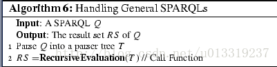
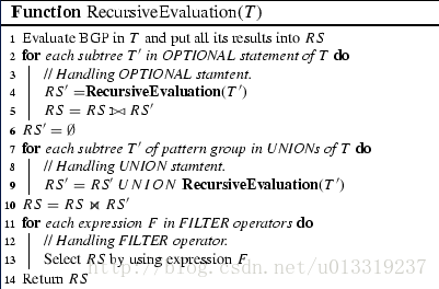
6 Handling general SPARQL

目前只讨论了basic graph pattern (BGP) query evaluation. 本节讨论如何扩展至general SPARQL queries involving UNION, OPTIONAL and FILTER statements.
DeFinition 15
(General SPARQL query) Any BGP is a SPARQL query. If $Q_1$ and $Q_2$ are SPARQL queries, then expressions $(Q_1 AND Q_2), (Q_1 UNION Q_2), (Q_1 OPT Q_2) and (Q_1 FILTER F)$ are also SPARQL queries.
Definition 16
(Match of general SPARQL query) Given an RDF graph G, the match set of a SPARQL query Q over G, denoted as [[Q]], is defined recursively as follows:

1. If Q is a BGP, [[Q]] is the set of matches defined in Definition 3 of Section 3.
2. If Q=$Q_1 AND Q_2$, then [[Q]]=$[[Q_1]]\bowtie [[Q_2]]$
3. If Q=$Q_1 UNION Q_2$, then [[Q]]=$[[Q_1]]\cup [[Q_2]]$
4. If Q=$Q_1 OPT Q_2$, then [[Q]]=$([[Q_1]]\bowtie [[Q_2]])\cup([[Q_1]]\ [[Q_2]])$
5. If Q=$Q_1 FILTER F$, then [[Q]]=$[[ Q ]] = \varTheta _F ([[ Q_1 ] ])$

7 Experiments

与其他方法做对比。a cloud-based approach (EAGRE), two partition-based approaches (Graphpartition and TripleGroup), two memory-based systemds (TriAD and Trinity.RDF) and two federated SPARQL query systems (FedX and SPLENDID).

7.1 Setting

We use two benchmark datasets with different sizes and one real dataset in our experiments, in addition to FedBench used in federated system experiments. Table 1 summarizes the statistics of these datasets.

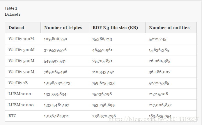
1. WatDiv is a benchmark that enables diversified stress testing of RDF data management systems.把不同大小的数据集随机分成N（N=10）份。（除了在实验六中）
2. LUBM is a bench mark that adopts an ontology for the university domain and can generate synthetic OWL data scalable to an arbitrary size. 使用了7个benchmark查询。
3. BTC 2012 is a real dataset that serves as the basis of submissions to Billion Triples Track of the Semantic Web Challenge.
4. FedBench is used for testing against federated systems.
实验环境：
a cluster of 10 machines running Linux, each of which has one CPU with four cores of 3.06 GHz, 16 GB memory and 500 GB disk storage.
Each site holds one fragment of the dataset. At each site, we install gStore to find inner matches, since it supports the graph-based SPARQL evaluation paradigm.
We use MPICH-3.0.4 library for communication.

7.2 Exp1: Evaluating each stage’s performance

In this experiment, we study the performance of our system at each stage (i.e., partial evaluation and assembly process) with regard to different queries in WatDiv 1B and LUBM 1000.
下面是具体的report, snowflake——several stars linked by a path.
complex——a combination of the above with complex structure.

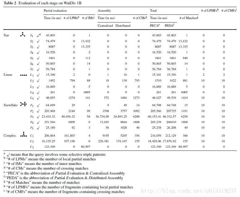
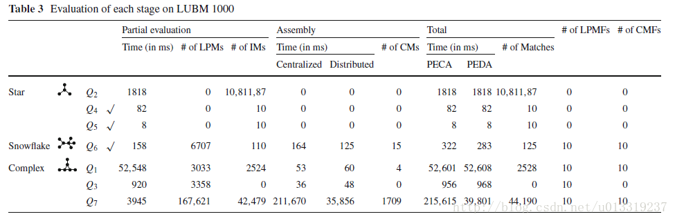
7.2.1 Partial evaluation

Tables 2 and 3 show that if there are some selective triple patterns10 in the query, the partial evaluation is much faster than others.
More inner matches and local partial matches lead to higher running time in the partial evaluation stage.

7.2.2 Assembly

We find that distributed assembly can beat the centralized one when there are lots of local partial matches and crossing matches.
大量的LPM送至server，server的处理能力达到了瓶颈。
大部分都涉及了所有的fragments。

7.3 Exp 2: Evaluating optimizations in assembly

In this experiment, we use WatDiv 1B to evaluate two different optimization techniques in the assembly: partitioning-based join strategy (Sect. 5.1) and the divide-and-conquer approach in the distributed assembly (Sect. 5.3).

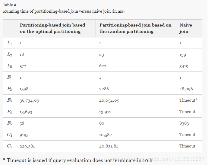
7.3.1 Partitioning-based join

First, we compare partitioning-based join (i.e., Algorithm 3) with naive join processing (i.e., Algorithm 2) in Table 4, which shows that the partitioning-based strategy can greatly reduce the join cost.
Second, we evaluate the effectiveness of our cost model. 即最佳划分的组装比随机划分的组装要快。

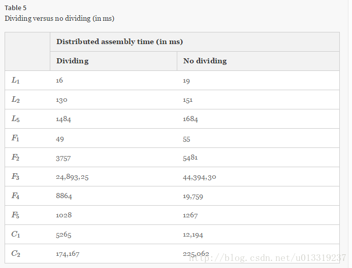
7.3.2 Divide-and-conquer in distributed assembly

Table 5 shows that dividing the search space will speed up distributed assembly.

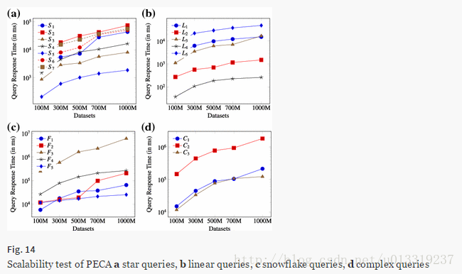
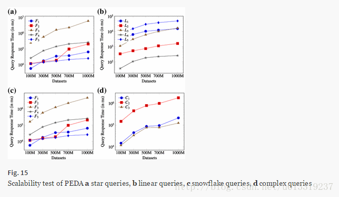
7.4 Exp 3: Scalability test

In this experiment, we vary the RDF dataset size from 100 million triples (WatDiv 100M) to 1 billion triples (WatDiv 1B) to study the scalability of our methods.
Query response time is affected by both the increase in data size (which is 1x→10x in these experiments) and the query type.

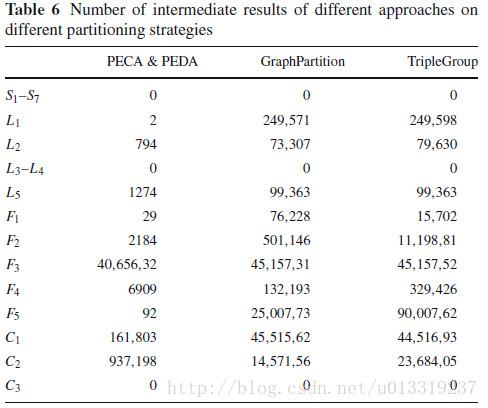
7.5 Exp 4: Intermediate result size and query performance versus query decomposition approaches

Table 6 compares the number of intermediate results in our method with two typical query decomposition approaches, i.e., GraphPartition and TripleGroup.
More intermediate results typically lead to more assembly time. Table 7 shows that our query response time is faster than others.


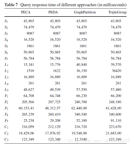
Our technique is always faster regardless of the use of MPI or MapReduce-based join.
Our partial evaluation process is more expensive in evaluating local queries than GraphPartition and TripleGroup in many cases.
Our system generally outperforms GraphPartition and TripleGroup significantly if they use MapReduce-based join. Even when GraphPartition and TripleGroup use distributed joins, our system is still faster than them in most cases.

7.6 Exp 5: Performance on RDF datasets with one billion triples

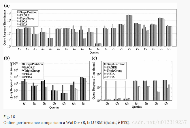
This experiment is a comparative evaluation of our method against GraphPartition, TripleGroup and EAGRE on three very large RDF datasets with more than one billion triples, WatDiv 1B, LUBM 10000 and BTC.
一半左右的query没有中间结果生成，所以差别不大。但其他的query本方法优势明显。
EAGRE stores all triples as flat files in HDFS and answers SPARQL queries by scanning the files. 所以比较耗时。但我们使用图匹配去响应查询，避免了对整个数据集的扫描。

7.7 Exp 6: Impact of different partitioning strategies

In this experiment, we test the performance under three different partitioning strategies over WatDiv 100 M.


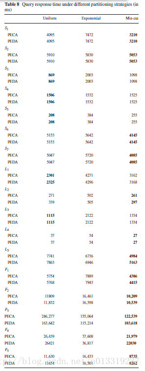
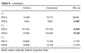
We implement three partitioning strategies: uniformly distributed hash partitioning, exponentially distributed hash partitioning, and minimum-cut graph partitioning.
The first partitioning strategy uniformly hashes a vertex v in RDF graph G to a fragment.
The second strategy uses an exponentially distributed hash function with a rate parameter of 0.5.
Minimum-cut partitioning strategy generally leads to fewer crossing edges than the other two.
Although our partial evaluation and assembly framework is agnostic to the particular partitioning strategy, it is clear that it works better when fragment sizes are balanced, and the crossing edges are minimized.

7.8 Exp 7: Comparing with memory-based distributed RDF systems

We compare our approach (which is disk-based) against TriAD and Trinity.RDF that are memory-based distributed systems. Our system is faster.

7.9 Exp 8: Comparing with federated SPARQL systems

We compare our methods with some federated SPARQL query systems including (FedX and SPLENDID).

7.10 Exp 9: Comparing with centralized RDF systems

和RDF-3X在LUBM 10000数据集上作比较。

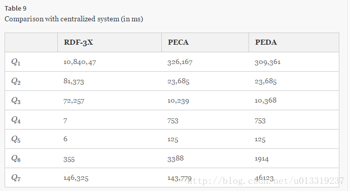
当查询比较复杂的时候，我们的方法优于RDF-3X。如果查询包含selective triple pattern，搜索空间比较小，则RDF-3X更快。

8 Conclusion

In this paper, we propose a graph-based approach to distributed SPARQL query processing that adopts the partial evaluation and assembly approach.
第一步，在每个段上对查询Q进行评估找到local partial matches.
第二步，组装这些local partial matches.两种方法
集中式组装：所有的local partial matches都发送至一个站点。
分布式组装：local partial matches在许多站点同时组装。
本方法的优点有两个：
一、本方法与分区方式无关，更加灵活。
二、中间结果比较少，和基于分区的方法相比。

下一步的工作：处理在linked open data (LOD)上的SPARQL queries。以及在分布式RDF图中的多重SPARQL查询优化。