Windows Graphviz | 安装 / 配置 / 绘图应用

注意：本文为 “Graphviz 在 Windows 系统中的安装、配置与绘图应用” 相关文章合辑。

中文引文，略作重排，未整理去重。
英文引文，机翻未校。

---

Windows 下 Graphviz 安装及入门教程

五道口纳什 于 2015-10-28 18:33:46 发布

发现好的工具，如同发现新大陆。有时，我们会好奇，论文中、各种专业书籍中那些形象的插图是如何制作出来的，这无一例外是对绘图工具的熟练运用。

Graphviz 是一个开源工具，可以在类似于 UNIX® 的大多数平台以及 Microsoft® Windows® 上运行。适用于大多数平台的二进制文件可以在 Graphviz 主页 上找到。AIX 二进制文件可以在 perzl.org 上找到。

Graphviz 应用程序中包含多种工具，用于生成各种类型的图表（如 dot、neato、circo、twopi 等）。本文将重点介绍用于生成层级图的 dot 工具。

工具名称	特点
dot	渲染的图具有明确的方向性。
neato	渲染的图缺乏方向性。
twopi	渲染的图采用放射性布局。
circo	渲染的图采用环型布局。
fdp	渲染的图缺乏方向性。
sfdp	渲染大型图，图片缺乏方向性。

下载安装及配置步骤简要

在 Windows 系统上安装配置 Graphviz

1. 下载安装包
   下载地址：Download | Graphviz
   双击 msi 文件，然后一直选择“下一步”（默认安装路径为 C:\Program Files (x86)\Graphviz2.38\）。安装完成后，将在 Windows 开始菜单创建快捷方式。

2. 配置环境变量
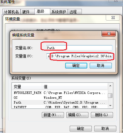
   计算机 → 属性 → 高级系统设置 → 高级 → 环境变量 → 系统变量 → Path
   在 Path 中加入路径：C:\Program Files (x86)\Graphviz2.38\bin

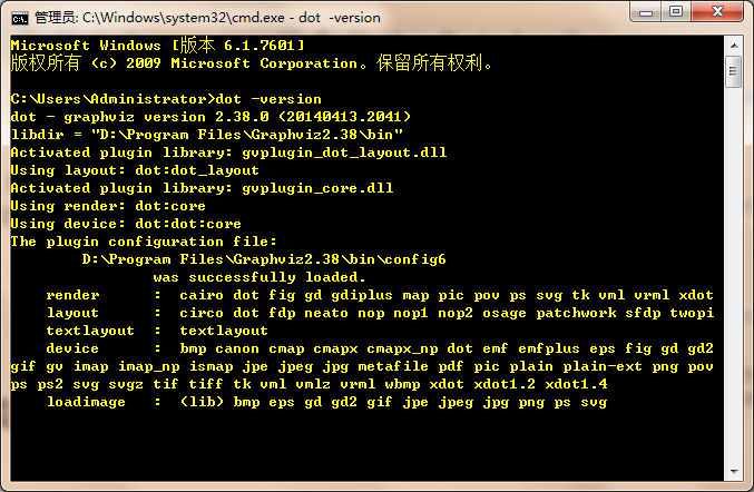
3. 验证
   在 Windows 命令行界面，输入 dot -version，然后按回车。如果显示 Graphviz 的相关版本信息，则安装配置成功。

---

下载安装及配置环境变量

安装

Windows 版本下载地址：Download

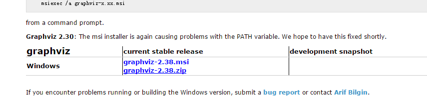
双击 msi 文件，然后一直选择“下一步”（记住安装路径，后续配置环境变量会用到）。安装完成后，将在 Windows 开始菜单创建快捷方式，默认快捷方式不会放在桌面。

配置环境变量

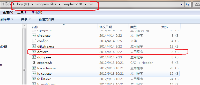
将 Graphviz 安装目录下的 bin 文件夹添加到 Path 环境变量中：

验证

进入 Windows 命令行界面，输入 dot -version，然后按回车。如果显示 Graphviz 的相关版本信息，则安装配置成功。

---

基本绘图入门

打开 Windows 下的 Graphviz 编辑器 gvedit，编写如下 dot 脚本语言，保存为 .gv 格式的文本文件。然后进入命令行界面，使用 dot 命令将 .gv 文件转换为 .png 图形文件。

dot D:\test\1.gv -Tpng -o image.png

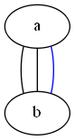
graph 示例

graph 使用 -- 描述关系：

graph pic1 {
  a -- b
  a -- b
  b -- a [color=blue]
}

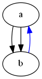
digraph 示例

digraph 使用 -> 描述关系：

digraph pic2 {
  a -> b
  a -> b
  b -> a [style=filled color=blue]
}

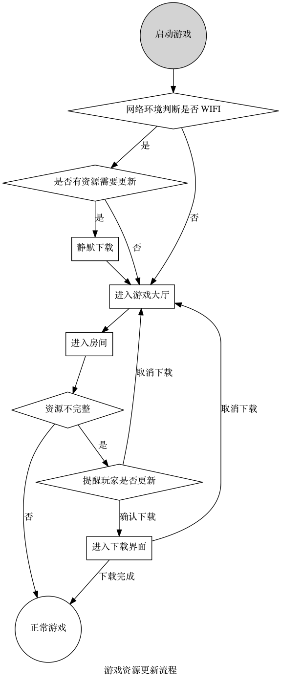
一个复杂的例子

digraph startgame {
    label="游戏资源更新流程"
    rankdir="TB"
    start [label="启动游戏" shape=circle style=filled]
    ifwifi [label="网络环境判断是否 WIFI" shape=diamond]
    needupdate [label="是否有资源需要更新" shape=diamond]
    startslientdl [label="静默下载" shape=box]
    enterhall [label="进入游戏大厅" shape=box]

    enterroom [label="进入房间" shape=box]
    resourceuptodate [label="资源不完整" shape=diamond]
    startplay [label="正常游戏" shape=circle fillcolor=blue]
    warning [label="提醒玩家是否更新" shape=diamond]
    startdl [label="进入下载界面" shape=box]
    //{rank=same; needupdate, enterhall}

    {shape=diamond; ifwifi, needupdate}

    start -> ifwifi
    ifwifi->needupdate [label="是"]
    ifwifi->enterhall [label="否"]
    needupdate->startslientdl [label="是"]
    startslientdl->enterhall
    needupdate->enterhall [label="否"]

    enterhall -> enterroom
    enterroom -> resourceuptodate
    resourceuptodate -> warning [label="是"]
    resourceuptodate -> startplay [label="否"]
    warning -> startdl [label="确认下载"]
    warning -> enterhall [label="取消下载"]
    startdl -> enterhall [label="取消下载"]
    startdl -> startplay [label="下载完成"]
}

---

与 Python 交互

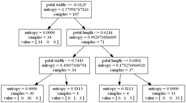
Graphviz 强大而便捷的关系图 / 流程图绘制方法，很容易让我们联想到机器学习中的 Decision Tree 的展示方式。幸运的是，scikit-learn 提供了生成 .dot 文件的接口，具体操作如下：

在 Python 编辑环境下：

from sklearn.tree import export_graphviz  # 导入的是一个函数
# tree 表示已经训练好的模型，即已经调用过 DecisionTreeClassifier 实例的 fit(X_train, y_train) 方法
export_graphviz(tree, out_file='tree.dot',
                feature_names=['petal length', 'petal width'])

进入 Windows 命令行界面，切换到 tree.dot 所在路径，执行：

dot -Tpng tree.dot -o tree.png

---

Graphviz 安装向导及入门指南

No_one-_-2022 于 2022-12-26 10:46:40 修改

1. 在官网下载 Graphviz

下载网址：Download | Graphviz

根据自身电脑位数选择合适的下载地址。

2. 安装

打开第一步下载好的软件，点击“下一步”。在安装路径选择时，可将安装路径修改为 E:\Graphviz。

注意：必须将 Graphviz 添加到系统 PATH 中。

选择好安装目录后，点击“下一步”，即可安装成功。

验证 PATH 是否正确添加到系统中。

可以看到 bin 文件夹已经添加到环境变量中。

3. 测试并在 Windows 命令行中使用

测试是否安装成功，可以通过 Win+R 或在搜索栏打开命令提示符窗口。

输入 dot -version（注意 dot 后面有一个空格）。如果成功出现如下信息，则表示安装成功。如果出现“dot 不是内部或外部命令”，则表示安装失败。

在桌面上保存一个 test.dot 文件，在命令行中调用如下命令：

dot -Tpng test.dot -o test.png

可以看到桌面上生成了 test.png 文件。

打开 test 的属性，可以看到文件类型是 DOT 文件。可以用 Windows 自带的文本编辑器打开，但必须另存为 DOT 文件，否则会出现错误：

dot: can't open test.dot

4. 在 Python 中使用

在命令行输入如下指令：

pip install graphviz

5. 在自带的 gvedit.exe 程序中使用

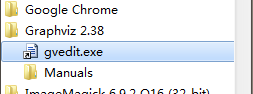
在 Windows 的所有程序中，找到以 G 开头的文件夹，点击打开 gvedit.exe。该程序是随 Graphviz 一起安装到电脑中的。注意程序需要下载 MSI 资源。

graphviz-2.37.20140115.zip - CSDN 下载

双击会弹出如下界面：

牢记一点：DOT 语言是一种工具，我们的目的是为了能够画出自己想要的图片，不要舍本逐末。

6. 在语雀中使用

语雀自带了文本绘图功能，非常方便。

7. 绘制一棵简单的二叉树

digraph BinaryTree  {
    a -> b
    a -> c
    b -> d
    d [label="null"];
    node1 [shape=point, style=invis]
    b -> node1 [weight=10, style=invis]
    b -> e
    c -> f
    node2 [shape=point, style=invis]
    c -> node2 [weight=10, style=invis]
    c -> g
    g [label="null"];
    e -> h
    h [label="null"];
    node3 [shape=point, style=invis]
    e -> node3 [weight=10, style=invis]

    e -> i
    i [label="null"];
    f -> k
    k [label="null"];
    node4 [shape=point, style=invis]
    f -> node4 [weight=10, style=invis]
    f -> j
    j [label="null"];
}

8. 详细语法介绍

8.1 带标签

digraph {
    player [label = "player"];
    game [label = "game"];
    player -> game [label = "play"]
}

8.2 修改方框颜色和形状

digraph {
    player [label = "player", color = Blue, fontcolor = Red, fontsize = 24, shape = box];
    game [label = "game", color = Red, fontcolor = Blue, fontsize = 24, shape = ellipse];
    player -> game [label = "play"]
}

详细信息可参考官方文档：Graphviz Shapes

8.3 子视图

digraph {
    label = visitNet
    rankdir = LR
    node [color = Red, fontsize = 24, shape = box]
    edge [color = Blue, style = "dashed"]
    user [style = "filled", color = "yellow", fillcolor = "chartreuse"]
    subgraph cluster_cd {
        label = "server and browser"
        bgcolor = yellow;
        browser -> server
    }
    user -> computer;
    computer -> browser;
}

8.4 结构视图

digraph {
    node [shape = record];
    struct1 [label = "<f0> left|<f1> mid\ dle|<f2> right"];
    struct2 [label = "<f0> one|<f1> two"];
    struct3 [label = "hello\nworld | {b|{c|<here> d|e}|f}|g|h"];
    struct1:f1 -> struct2:f0;
    struct1:f2 -> struct3:here;
}

8.5 继承关系

digraph UML {

    node [fontname = "Courier New", fontsize = 10, shape = record];
    edge [fontname = "Courier New", fontsize = 10, arrowhead = "empty"];

    Car [label = "{Car | v : float\nt : float | run () : float}"]

    subgraph clusterSome {
        bgcolor = "yellow";
        Bus [label = "{Bus | | carryPeople () : void}"];
        Bike [label = "{bike | | ride () : void}"];
    }
    Bus -> Car
    Bike -> Car
}

---

GraphViz 使用教程 - 用代码生成有向图。并介绍流程图、时序图等绘图工具

youwen21 于 2019-08-10 15:46:03 发布

GraphViz 简述

GraphViz 是一个使用 DOT 编程语言生成有向图，无向图等图象的工具。 如果只是偶尔使用，可以在本地先定义好关系，使用 web 浏览器在线生成关系图。

GraphViz 基本元素

• (N) node 节点
• (E) edge 线
• (G) graph 图
• (S) subgraph 子图
• © cluster subgraphs 子图群

生成一个有向图

第一步，定义关系如下：

总部->{市场营销部;财务部;人力行政部;技术部;}
技术部->{后端开发;前端开发;运维;}
市场营销部->{线下营销; 线上营销}

第二步，给定义好的关系起个名字，一个有向图定义完成

digraph 组织架构{
总部->{市场营销部;财务部;人力行政部;技术部;}
技术部->{后端开发;前端开发;运维;}
市场营销部->{线下营销; 线上营销}
}

组织架构，函数调用，物流追踪，网络追踪，审批流程等有向操作，只需要用 “->” 定义节点之间的关系，便可以生成其关系图。
复杂的节点关系用 graphviz 生成图可更直观地观察节点之间的关系。

node 属性、edit 属性和 subgraph 的使用

digraph {
	bgcolor="#EEEEEE";

	node [shape="box"];
	a[shape="ellipse", color="red"];
	b[fontcolor="#55AA55", style="dotted"];
	c[style="invis"];
	d[style="filled" color="#F9B34B"];
	stract_z[shape="record", label="<f1> 第一列|{<f21> 第二列-行| <f22> 第二列二行}|<f3> 第三列"];

	a->stract_z:f21;
	b->stract_z:f22[style="dotted", color="#55AA55"];
	a->c[headclip=false, arrowhead="none"];
	c->d[tailclip=false];
	d->sa:sa01;

	subgraph cluster_a {
		label="定义的一个子图";
		style="rounded"
		sa[shape="record", label="{{<sa01> 001 | <sa02> 002}|<sa1> sa1| <sa2> sa2}"];
		sa:sa1->sb;
		sa:sa2->sc;
	}

	{rank="same"; stract_z; d}
}

上面的例包含了常用的定义 node 节点内容和样式和颜色， edge 样式和颜色，隐藏 node，子图，PORT 链接点和节点同级。
总得来说，用 GraphViz 画有向图只需要定义节点和节点关系即可，样式等其他无关紧要的东西并不常用，可慢慢调整。

如何安装 GraphViz

GraphViz 支持 Linux , Windows , Mac 系统平台 。如 mac 用 brew 安装

brew install graphviz

Linux , Windows 平台到官方网站找相应的安装包。

下载地址： https://www.graphviz.org/download

GraphViz 工具

GraphViz 支持的命令有

• dot − filter for drawing directed graphs
• neato − filter for drawing undirected graphs
• twopi − filter for radial layouts of graphs
• circo − filter for circular layout of graphs
• fdp − filter for drawing undirected graphs
• sfdp − filter for drawing large undirected graphs
• patchwork − filter for squarified tree maps
• osage − filter for array-based layouts

本文讲述 dot 有向图的使用

dot 命令行调用

//dot -Tpng -o a.png a.dot && open a.png
dot -Tpng -o a.png a.dot

配置 Sublime 支持图片预览

此安装方式，需要 Sublime 已经安装了 Package Control

• command+shift+p 打开命令面板
• package install GraphvizPreview
  安装成功后，按快捷 control+shift+g 便可为当前打开的 dot 文件生成预览图

精通 sublime 的话，可以自已配置 Build System 的方式实现生成图片

web 端在线生成图片

在线生成有向图：
https://graphviz.herokuapp.com/

你也可以搭建自己专用的 webgraph 编辑器，git 仓库地址：
https://github.com/Potherca/GraphvizWebEditor

克隆到网站目录下执行 composer install 便可以使用。

桌面端应用

DotEditor

其他图象化工具

• PlantUML - 时序图，用例图，类图，组件图，等程序架构图绘制工具（PlantUML 可以以 jar 包的方式运行，底层调用 GraphViz 生成图象）
• D3 vs G2 vs Echarts - javascript 前端绘图工具
• Neo4j - NOSQL 图形数据库
• Xmind - 脑图工具

在线绘图工具

• ProcessOn思维导图流程图-在线画思维导图流程图_在线作图实时协作
  https://www.processon.com/
• 百度脑图 - 便捷的思维工具
  https://naotu.baidu.com/
• draw.io
  https://www.draw.io/
• The Simplest Flowchart Maker | Free & Online Creator
  https://www.zenflowchart.com/
• Communicate Complexity With Intuitive Diagramming | Gliffy by Perforce
  https://www.gliffy.com/

---

Let’s Draw a Graph: An Introduction with Graphviz

使用 Graphviz 画图介绍

Marc Khoury

Electrical Engineering and Computer Sciences University of California at Berkeley
加州大学伯克利分校电气工程与计算机科学系

Technical Report No. UCB/EECS-2013-176
技术报告编号：UCB/EECS-2013-176

http://www.eecs.berkeley.edu/Pubs/TechRpts/2013/EECS-2013-176.html

October 28, 2013

Copyright © 2013, by the author(s). All rights reserved. Permission to make digital or hard copies of all or part of this work for personal or classroom use is granted without fee provided that copies are not made or distributed for profit or commercial advantage and that copies bear this notice and the full citation on the first page. To copy otherwise, to republish, to post on servers or to redistribute to lists, requires prior specific permission.

1 Introduction

引言

Graphs are ubiquitous data structures in computer science. Many important problems have solutions hidden in the complexity of modern graphs, rendering effective visualization techniques extremely valuable. The need for such visualization techniques has led to the creation of a myriad of graph drawing algorithms. We present several algorithms to draw several of the most common types of graphs. We will provide instruction in the use of Graphviz, a popular open-source graph drawing package developed at AT&T Labs, to execute these algorithms. All figures shown herein were generated with Graphviz.
图是计算机科学中无处不在的数据结构。许多重要问题的解决方案隐藏在现代图的复杂性中，使得有效的可视化技术极为有价值。这种可视化技术的需求促使了大量图绘制算法的诞生。我们介绍了几种用于绘制最常见类型的图的算法，并将指导如何使用 Graphviz，这是一个由 AT&T 实验室开发的流行的开源图绘制工具包，来执行这些算法。本文中展示的所有图形都是通过 Graphviz 生成的。

2 The DOT Language

DOT 语言

Visualization of a given graph requires that it first be represented in a format understandable by graph drawing packages. We will use the DOT format, a format that can encode most attributes of a graph in a human-readable manner [1].
要可视化一个给定的图，需要先将其表示为图绘制工具包能够理解的格式。我们将使用 DOT 格式，这种格式能够以人类可读的方式编码图的大部分属性 [1]。

2.1 Undirected Graphs

无向图

A DOT file for an undirected graph begins with the keyword graph followed by the name of the graph. An undirected edge between vertices u and v can be specified by u–v. A simple example of an undirected graph with five vertices and five edges is illustrated by Figure 1, below.
无向图的 DOT 文件以关键字 graph 开始，后跟图的名称。顶点 u 和 v 之间的无向边可以通过 u--v 指定。下面的图 1 展示了一个包含五个顶点和五条边的无向图的简单示例。

Listing 1: A DOT file for a simple undirected graph with five vertices.

列表 1：一个包含五个顶点的简单无向图的 DOT 文件。

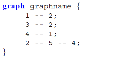
graph graphname {
	1 -- 2; 
	3 -- 2; 
	4 -- 1;
	2 -- 5 -- 4;
}

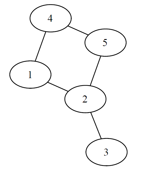
Figure 1: Visualization of Listing 1 graph.
图 1：列表 1 图的可视化。

The Graphviz application neato is a straightforward method of rapidly visualizing undirected graphs in the format described above. Figure 1 was generated by the command neato -Teps undirected.gv > undirected.eps, where undirected.gv is a file containing the code shown in Figure 1 and -Teps specifies an Encapsulated Postscript output format. Graphviz supports a wide range of output formats including GIF, JPEG, PNG, EPS, PS, and SVG. All Graphviz programs perform I/O operations on standard input and output in the absence of specified files.
Graphviz 的 neato 应用程序是一种快速可视化上述格式无向图的简单方法。图 1 是通过命令 neato -Teps undirected.gv > undirected.eps 生成的，其中 undirected.gv 是包含图 1 所示代码的文件，-Teps 指定了封装 Postscript 输出格式。Graphviz 支持包括 GIF、JPEG、PNG、EPS、PS 和 SVG 在内的广泛输出格式。在没有指定文件的情况下，所有 Graphviz 程序都在标准输入和输出上执行 I/O 操作。

2.2 Directed Graphs

A directed graph begins with the keyword digraph followed by the name of the graph. A directed edge between two vertices u and v is specified by u->v. The aforementioned edge starts at u and goes to v. The DOT code for and visualization of an example directed graph appears in Listing 2 and Figure 2, respectively. The visualization in Figure 2 was produced via the command dot -Teps directed.gv > directed.eps.
有向图以关键字 digraph 开始，后跟图的名称。两个顶点 u 和 v 之间的有向边通过 u->v 指定。上述边从 u 开始，指向 v。示例有向图的 DOT 代码和可视化分别出现在列表 2 和图 2 中。图 2 的可视化是通过命令 dot -Teps directed.gv > directed.eps 生成的。

Listing 2: A DOT file for a simple directed graph.
列表 2：一个简单有向图的 DOT 文件。

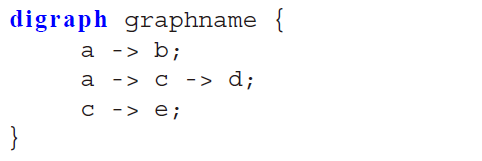
digraph graphname {
	a -> b; 
	a -> c -> d; 
	c -> e;
}

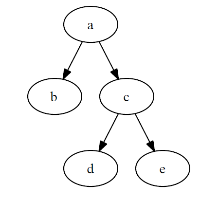
Figure 2: Visualization of Listing 2 graph.
图 2：列表 2 图的可视化。

2.3 Attributes

The DOT format supports a wide selection of attributes for vertices, edges, and graphs. Examples of user-definable attributes include the color and shape of a vertex or the weight and style of an edge. There are far too many attributes to list here and we direct the reader to the Graphviz documentation for a comprehensive list. Graphviz defines default values for most of the attributes available for DOT files. Many attributes are only used by specific Graphviz programs. As an example, the repulsive force attribute is only used by the sfdp module.
DOT 格式支持大量顶点、边和图的属性。用户可定义的属性示例包括顶点的颜色和形状或边的权重和样式。这里无法列出所有属性，我们建议读者查阅 Graphviz 文档以获取完整的列表。Graphviz 为 DOT 文件可用的大多数属性定义了默认值。许多属性仅被特定的 Graphviz 程序使用。例如，斥力属性仅由 sfdp 模块使用。

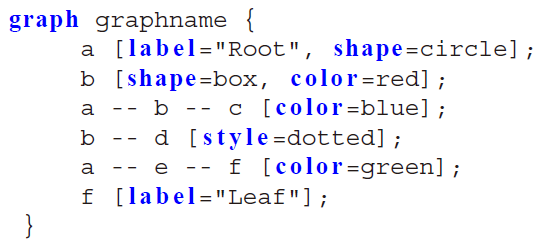
Listing 3: A DOT file where most vertices and edges have been assigned various attributes.
列表 3：大多数顶点和边都被分配了各种属性的 DOT 文件。

graph graphname {
	a [label ="Root", shape=circle]; 
	b [shape=box, color=red]; 
	a -- b -- c [color=blue];
	b -- d [style =dotted]; 
	a -- e -- f [color=green]; 
	f [ label ="Leaf"];
}

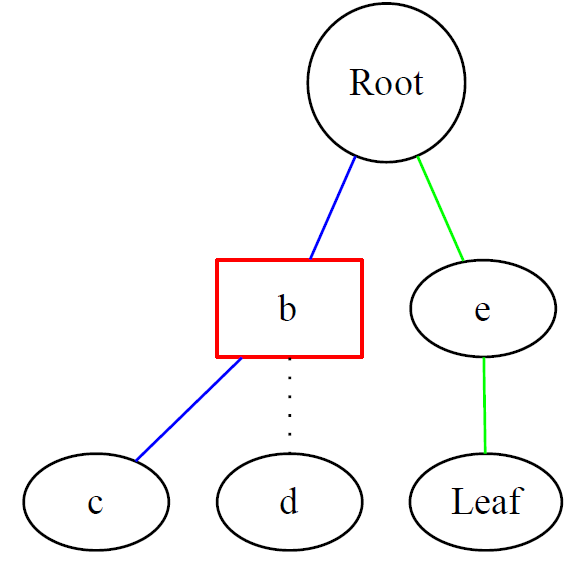
Figure 3: Visualization of Listing 3 graph.

图 3：列表 3 图的可视化。

Attributes may be used to draw attention to sections of a graph (e.g. color and thickness adjustment to highlight a path).

属性可用于突出显示图的某些部分（例如，通过调整颜色和粗细来突出路径）。

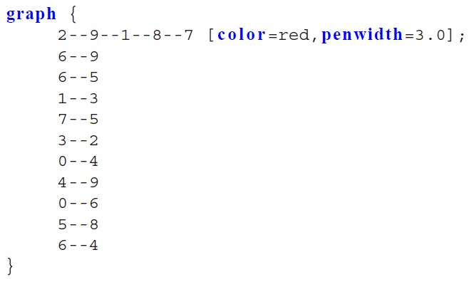
Listing 4: A DOT file where edges along a path have been colored red.

列表 4：路径上的边被涂成红色的 DOT 文件。

graph {
2 -- 9 -- 1 -- 8 -- 7 [color=red,penwidth=3.0]; 
6 -- 9
6 -- 5
1 -- 3 
7 -- 5
3 -- 2
0 -- 4
4 -- 9
0 -- 6
5 -- 8
6 -- 4
}

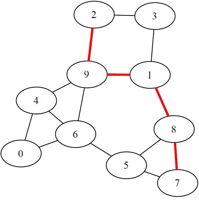
Figure 4: Visualization of Listing 4 graph.

图 4：列表 4 图的可视化。

2.4 Clustering

In some graphs, grouping of vertex subsets is desirable. This grouping of vertex subsets is particularly useful in the case of k-partite graphs. The DOT language allows the specification of subgraphs which can be clustered together and visually separated from other parts of the graph. In a graph file the keyword subgraph is used to specify a subgraph. Prefacing the name of the subgraph with the expression “cluster ” ensures that the subgraph will be visually separated in the layout. Note that only dot and fdp (explained in detail later in this document) support clustering. Figure 5 was generated by the command dot -Teps cluster.gv > cluster.eps.

在某些图中，对顶点子集进行分组是可取的。这种顶点子集的分组在 k-部图中尤其有用。DOT 语言允许指定可以聚集在一起并在布局中与其他部分视觉上分开的子图。在图文件中，使用关键字 subgraph 来指定子图。在子图名称前加上表达式 “cluster” 可确保子图在布局中被视觉上分开。请注意，只有 dot 和 fdp（本文稍后将详细介绍）支持聚类。图 5 是通过命令 dot -Teps cluster.gv > cluster.eps 生成的。

Listing 5: A graph with two clusters representing different processes.
列表 5：一个包含两个分别代表不同进程的聚类的图。

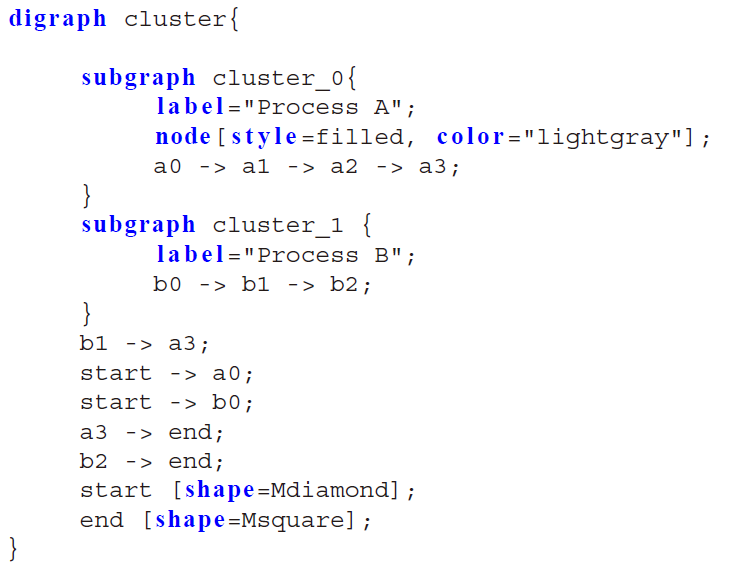
digraph cluster{
		subgraph cluster_0{
			label ="Process A";
			node[ style =filled, color="lightgray"];
			a0 -> a1 -> a2 -> a3;
	}
	subgraph cluster_1 {
			label ="Process B";
			b0 -> b1 -> b2;
	}
	b1 -> a3;
	start -> a0;
	start -> b0;
	a3 -> end;
	b2 -> end;
	start [shape=Mdiamond];
	end [shape=Msquare];
}

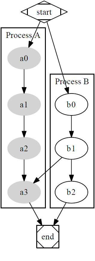
Figure 5: Visualization of Listing 5 graph.
图 5：列表 5 图的可视化。

3 Force-Directed Methods

Force-directed algorithms model graph layouts as physical systems, assigning attractive and repulsive forces between vertices and minimizing the total energy in the system. The optimal layout is defined as the layout corresponding to the global minimum energy. The spring-electrical model assigns two forces between vertices: the repulsive force $f_r$ and the attractive force $f_a$. The repulsive force is defined for all pairwise combinations of vertices and is inversely proportional to the distance between them. The attractive force exists only between neighboring vertices and is proportional to the square of the distance. Intuitively, every vertex wants to keep its neighbors close while pushing all other vertices away [7].

力导向算法将图布局建模为物理系统，在顶点之间分配吸引力和斥力，并最小化系统中的总能量。最优布局被定义为对应于全局最小能量的布局。弹簧 - 电气模型在顶点之间分配两种力：斥力 $f_r$ 和吸引力 $f_a$。斥力被定义为所有顶点对之间的力，并与它们之间的距离成反比。吸引力仅存在于相邻顶点之间，并与距离的平方成正比。直观上，每个顶点都希望保持其邻居靠近，同时将所有其他顶点推远 [7]。

$$f_r(i,j)=-\frac{C{K}^2}{\Vert x_i-x_j\Vert },i\ne j,i,j\in V\text{\hspace{1em}(1)}$$

$$f_a(i,j)=\frac{{\Vert x_i-x_j\Vert }^2}{K},(i,j)\in E\text{\hspace{1em}(2)}$$

The force on vertex $i$ is the sum of the attractive (from vertices $j\in V,j\ne i,(i,j)\in E$) and repulsive (from vertices $j\in V$) forces.

顶点 $i$ 上的力是吸引力（来自顶点 $j\in V,j\ne i,(i,j)\in E$）和斥力（来自顶点 $j\in V$）的总和。

$$f(i,K,C)=\sum _{j\ne i,j\in V}-\frac{C{K}^2}{\Vert x_i-x_j\Vert }(x_j-x_i)+\sum _{(i,j)\in E}\frac{{\Vert x_i-x_j\Vert }^2}{K}(x_j-x_i)\text{\hspace{1em}(3)}$$

The parameter $K$ is known as the optimal distance and the parameter $C$ is used to control the relative strength of the attractive and repulsive forces. While the choice of these parameters is important in practice, mathematically it can be shown that they only scale the layout [7]. Finally, the total energy in the system is the sum of the squared forces.

参数 $K$ 被称为最优距离，参数 $C$ 用于控制吸引力和斥力的相对强度。虽然在实践中选择这些参数很重要，但从数学上可以证明，它们只是对布局进行缩放 [7]。最后，系统中的总能量是力的平方和。

$$\text{energy}(K,C)=\sum _{i\in V}f(i,K,C{)}^2\text{\hspace{1em}(4)}$$

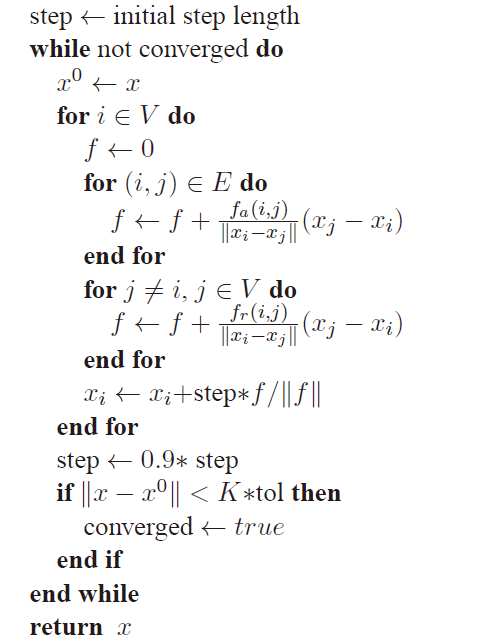
For each vertex $i$ the algorithm computes the forces acting on $i$ and adjusts the position of $i$ in the layout. The algorithm repeats this process until it converges on a final layout. The presented force-directed layout algorithm requires $O(V^2)$ time per iteration and it is generally considered that $O(V)$ iterations are required.

对于每个顶点 $i$，算法计算作用在 $i$ 上的力，并调整 $i$ 在布局中的位置。算法重复此过程，直到收敛到最终布局。所介绍的力导向布局算法每轮迭代需要 $O(V^2)$ 时间，通常认为需要 $O(V)$ 次迭代。

Algorithm 1 ForceDirectedLayout $(G,x,tol)$

算法 1：力导向布局（ForceDirectedLayout）

The Graphviz program fdp uses a force-directed algorithm to generate layouts for undirected graphs. fdp is suitable for small graphs that are both unweighted and undirected. Figure 6, below, displays a layout generated by fdp for a torus generated using the command fdp -Teps torus.gv > torus.eps.

Graphviz 的 fdp 程序使用力导向算法为无向图生成布局。fdp 适用于小型无权无向图。下面的图 6 展示了 fdp 为一个环面生成的布局，该布局是通过命令 fdp -Teps torus.gv > torus.eps 生成的。

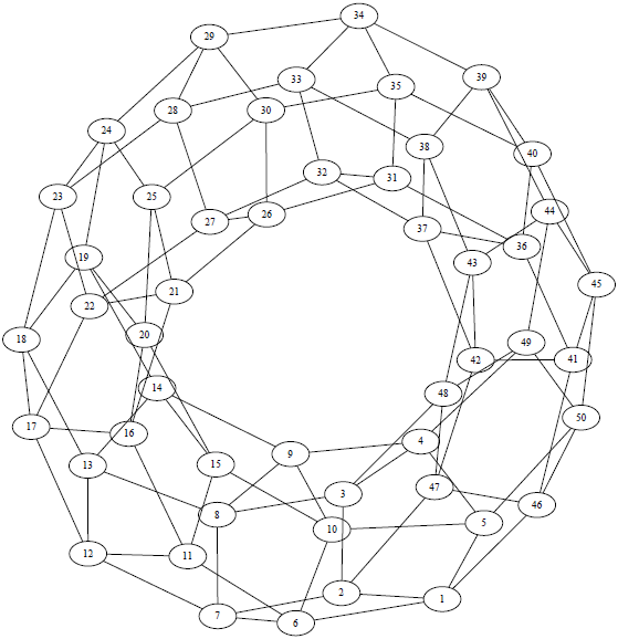
Figure 6: A drawing of a torus produced by fdp.
图 6：由 fdp 生成的环面绘制图。

The complexity of this computation can be decreased by employing a Barnes-Hut scheme to compute the forces acting on a vertex [2]. The use of a quadtree to group vertices into supernodes allows a single computation to approximate the force contributions of a large collection of vertices. This scheme reduces the complexity of the innermost loop from $O(V)$ to $O(\log (V))$, dropping the whole algorithm to $O(V\log (V))$ per iteration. The speed of this technique can be further improved by using a multilevel approach that takes advantage of graph coarsening techniques. The Graphviz program sfdp implements these techniques and is currently the optimal choice for generating large graph layouts.

通过使用 Barnes-Hut 方案计算作用于顶点的力，可以降低此计算的复杂度 [2]。使用四叉树将顶点分组成超节点，允许单次计算近似大量顶点的力贡献。这种方案将最内层循环的复杂度从 $O(V)$ 降低到 $O(\log (V))$，从而使整个算法的每轮迭代复杂度降至 $O(V\log (V))$。通过使用利用图简化技术的多级方法，可以进一步提高此技术的速度。Graphviz 的 sfdp 程序实现了这些技术，目前是生成大型图布局的最佳选择。

Figure 7: A drawing of a graph with 40000 vertices produced by sfdp.
图 7：由 sfdp 生成的包含 40000 个顶点的图的绘制图。

4 Stress Majorization

应力优化

Stress majorization attempts to embed the graph metric into ${\mathbb{R}}^k$ [5]. If the shortest path distance between two vertices $i,j\in V$ is $d_{ij}$, then stress majorization will attempt to place these two vertices at distance $d_{ij}$ apart in the layout. To accomplish this, stress majorization uses an iterative optimization process to find a global minimum of the stress function shown in Equation 5. The iterative equation involves two weighted Laplacian matrices. For a quick introduction to Laplacian matrices and their properties, please see Appendix A. Laplacian matrices permit many different types of weightings. Here we consider two weighted Laplacian matrices that are important for stress majorization. Let $d_{ij}$ be the shortest path distance - sometimes referred to as the “graph-theoretic distance” - between two vertices $i,j\in V$. Let $w_{ij}=d_{ij}^{-p}$ and choose $p=2$. Technically, $p$ could be any integer, but $p=2$ seems to produce the best graph drawings in practice.

应力主化方法试图将图度量嵌入到 ${\mathbb{R}}^k$ 中 [5]。如果两个顶点 $i,j\in V$ 之间的最短路径距离为 $d_{ij}$，那么应力主化将尝试在布局中将这两个顶点放置在距离 $d_{ij}$ 处。为了实现这一点，应力主化使用迭代优化过程来寻找应力函数（如公式 5 所示）的全局最小值。迭代方程涉及两个加权拉普拉斯矩阵。关于拉普拉斯矩阵及其性质的简要介绍，请参阅附录 A。拉普拉斯矩阵允许许多不同类型的权重。这里我们考虑两个对应力主化很重要的加权拉普拉斯矩阵。设 $d_{ij}$ 为两个顶点 $i,j\in V$ 之间的最短路径距离（有时也称为“图论距离”）。设 $w_{ij}=d_{ij}^{-p}$，并选择 $p=2$。从技术上讲，$p$ 可以是任何整数，但实践中 $p=2$ 似乎能产生最佳的图绘制效果。

Definition 1 Let $G$ be a graph and let $d$ be the shortest path distance matrix of $G$. Define $w_{ij}=d_{ij}^{-2}$. The weighted Laplacian $L_w$ of a graph $G$ is an $n\times n$ matrix given by:

定义 1：设 $G$ 是一个图，$d$ 是 $G$ 的最短路径距离矩阵。定义 $w_{ij}=d_{ij}^{-2}$。图 $G$ 的加权拉普拉斯矩阵 $L_w$ 是一个 $n\times n$ 矩阵，定义为：

$$L_w^{i,j}=\{\begin{array}{ll}-w_{ij}& \text{if }i\ne j\\ {\sum }_{k\ne i}{w}_{ik}& \text{if }i=j\end{array}$$

The off diagonal elements of the weighted Laplacian are $-w_{ij}$, as opposed to $-1$ and $0$. The diagonal element $L_w[i,i]$ is the positive sum of the off diagonal elements for row $i$, as with the standard Laplacian matrix. The second type of weighted Laplacian matrix that we will consider is weighted by a layout of the graph: the positions of the vertices in $k$-dimensional space. We denote a $k$-dimensional layout by an $n\times k$ matrix $X$. The position of the $i$-th vertex is $X_i\in {\mathbb{R}}^k$. Lastly define a function $\text{inv}(x)=\frac{1}{x}$ when $x\ne 0$ and $0$ otherwise.

加权拉普拉斯矩阵的非对角线元素是 $-w_{ij}$，而不是 $-1$ 和 $0$。对角线元素 $L_w[i,i]$ 是行 $i$ 中非对角线元素的正值和，与标准拉普拉斯矩阵相同。我们将考虑的第二种加权拉普拉斯矩阵是根据图的布局加权的：顶点在 $k$ -维空间中的位置。我们用一个 $n\times k$ 矩阵 $X$ 表示 $k$ -维布局。第 $i$ 个顶点的位置是 $X_i\in {\mathbb{R}}^k$。最后定义一个函数 $\text{inv}(x)=\frac{1}{x}$，当 $x\ne 0$ 时，否则为 $0$。

Definition 2 Let $G$ be a graph and let $X$ be a layout for $G$. The weighted Laplacian matrix $L_X$ is an $n\times n$ matrix given by:

定义 2：设 $G$ 是一个图，$X$ 是 $G$ 的一个布局。加权拉普拉斯矩阵 $L_X$ 是一个 $n\times n$ 矩阵，定义为：

$$L_w^{i,j}=\{\begin{array}{ll}-w_{ij}{d}_{ij}\text{inv}(\Vert X_i-X_j\Vert )& \text{if }i\ne j\\ -{\sum }_{k\ne i}{L}_X[i,k]& \text{if }i=j\end{array}$$

The off diagonal elements of $L_X$ are $-w_{ij}{d}_{ij}\text{inv}(\Vert X_i-X_j\Vert )$ where $\Vert X_i-X_j\Vert$ is the Euclidean distance between vertices $i$ and $j$ in the layout. The diagonal element $L_X[i,i]$ is the positive sum of the off diagonal elements in row $i$. The optimal layout corresponds to the global minimum of the following stress function.

$L_X$ 的非对角线元素是 $-w_{ij}{d}_{ij}\text{inv}(\Vert X_i-X_j\Vert )$，其中 $\Vert X_i-X_j\Vert$ 是布局中顶点 $i$ 和 $j$ 之间的欧几里得距离。对角线元素 $L_X[i,i]$ 是行 $i$ 中非对角线元素的正值和。最优布局对应于以下应力函数的全局最小值。

$$\text{stress}(x)=\sum _{i<j}{w}_{ij}(\Vert X_i-X_j\Vert -d_{ij}{)}^2\text{\hspace{1em}(5)}$$

The minimum of the stress is given by an iterative system involving weighted Laplacian matrices. Here $Z$ is the current layout and $X$ is the next layout. At the end of each iteration $X$ is assigned to $Z$ to compute a new $X$. The process continues until the stress function converges. A random layout can be used as the initial layout $Z$, but tends to require more iterations until convergence and is more likely to converge to a local minima.

应力的最小值由一个涉及加权拉普拉斯矩阵的迭代系统给出。这里 $Z$ 是当前布局，$X$ 是下一个布局。在每次迭代结束时，将 $X$ 赋值给 $Z$ 以计算新的 $X$。该过程一直持续到应力函数收敛为止。可以使用随机布局作为初始布局 $Z$，但通常需要更多次迭代才能收敛，并且更有可能收敛到局部最小值。

$$L^{w}X=L^{Z}Z\text{\hspace{1em}(6)}$$

Laplacian matrices are known to be positive-semidefinite with a one-dimensional null space spanned by $1=(1,1,\dots ,1)\in {\mathbb{R}}^n$. Intuitively, the null space tells us that our stress function is invariant under translation. To remove this degree of freedom, we remove the first row and column and consider only the $(n-1)\times (n-1)$ submatrix of each Laplacian matrix. This method requires us to set $X_0=0$ in the layout. As these submatrices are strictly diagonally dominant and positive-definite, we employ the conjugate gradient method to solve the system [9]. The conjugate gradient method is a popular algorithm for solving systems of linear equations of the form $A\mathbf{x}=\mathbf{b}$, where $\mathbf{x}$ is an unknown vector, $\mathbf{b}$ is a known vector, and $A$ is a known, square, symmetric, and positive-definite matrix. Stress majorization produces layouts that approximate the actual graph metric because it considers the graph-theoretic distance between every two vertices. This method can easily account for weighted edges or other desired graph metrics, providing a clear advantage over the previously described spring-electrical model. The requirement of access to the all-pairs shortest path matrix, $d$, severely constrains the scalability of stress majorization. Execution of Dijkstra’s algorithm at each vertex allows computation of the APSP matrix in $O(VE+V^2\log (V))$ time. Additionally, at each iteration we must compute $L_Z$, perform a matrix multiplication with $Z$, and use the conjugate gradient method to solve the system. As a result, stress majorization is not scalable beyond approximately $10^4$ vertices. Low-rank Laplacian matrices have recently been used to extend stress majorization to much larger graphs [8]. An upcoming version of Graphviz will include an implementation of this extension. Stress majorization is implemented in the Graphviz program neato. neato is suitable for weighted, or unweighted, undirected graphs.

拉普拉斯矩阵已知是半正定的，其一维零空间由 $1=(1,1,\dots ,1)\in {\mathbb{R}}^n$ 张成。直观上，零空间告诉我们，我们的应力函数在平移下是不变的。为了消除这一自由度，我们移除第一行和第一列，仅考虑每个拉普拉斯矩阵的 $(n-1)\times (n-1)$ 子矩阵。这种方法要求我们在布局中设置 $X_0=0$。由于这些子矩阵是严格对角占优且正定的，我们采用共轭梯度法来求解该系统 [9]。共轭梯度法是一种流行的算法，用于求解形式为 $A\mathbf{x}=\mathbf{b}$ 的线性方程组，其中 $\mathbf{x}$ 是未知向量，$\mathbf{b}$ 是已知向量，而 $A$ 是已知的、方阵的、对称的且正定的矩阵。应力主化方法产生的布局能够近似实际的图度量，因为它考虑了每两个顶点之间的图论距离。这种方法可以轻松地考虑加权边或其他期望的图度量，与前面描述的弹簧 - 电气模型相比具有明显优势。需要访问所有点对最短路径矩阵 $d$，这严重限制了应力主化的可扩展性。在每个顶点上执行 Dijkstra 算法可以在 $O(VE+V^2\log (V))$ 时间内计算 APSP 矩阵。此外，在每次迭代中，我们需要计算 $L_Z$，执行与 $Z$ 的矩阵乘法，并使用共轭梯度法求解系统。因此，应力主化无法扩展到大约 $10^4$ 个顶点以上的图。最近，低秩拉普拉斯矩阵被用来将应力主化扩展到更大的图 [8]。Graphviz 的一个即将发布的版本将包含这种扩展的实现。应力主化在 Graphviz 的 neato 程序中得以实现。neato 适用于加权或无权的无向图。

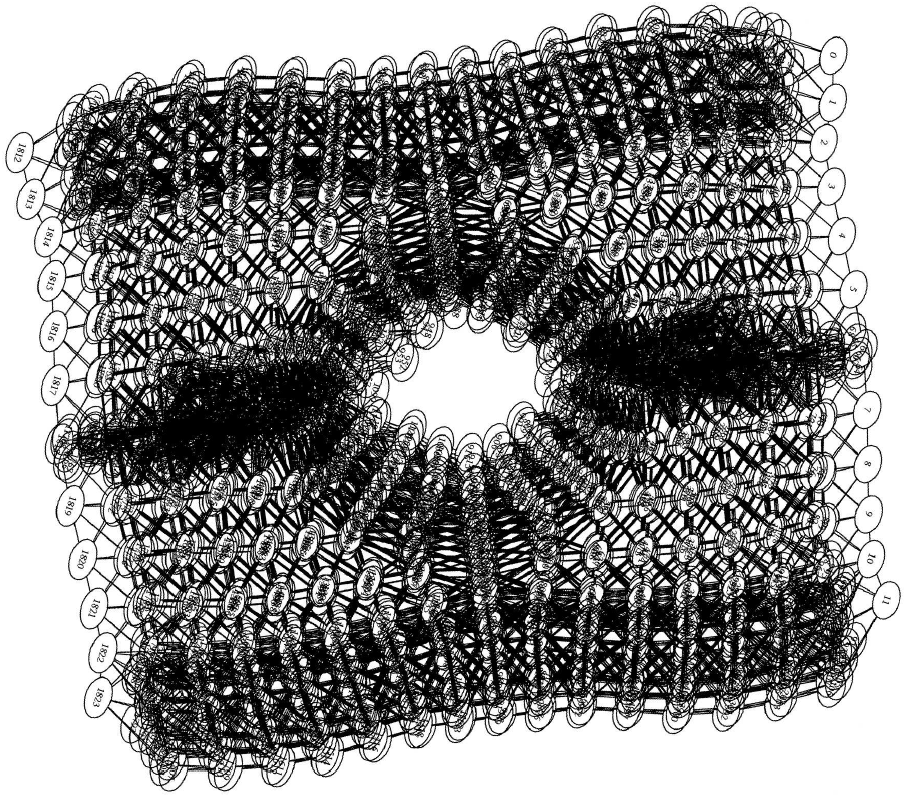
Figure 8: A drawing by neato of the nasa1824 dataset.
图 8：由 neato 绘制的 nasa1824 数据集。

5 Reducing Edge Crossings

减少边交叉

Thus far, we have limited our discussion to graph drawing algorithms for undirected graphs. Drawing directed graphs is an entirely new problem. The naive approach is to simply ignore the direction of the edges and use an algorithm for drawing undirected graphs. This is fundamentally unsatisfying because the directionality is frequently very important to effectively visualizing the graph.

到目前为止，我们的讨论仅限于无向图的绘制算法。绘制有向图是一个全新的问题。一种简单的方法是直接忽略边的方向，使用绘制无向图的算法。这种方法本质上是不令人满意的，因为方向性对于有效地可视化图通常非常重要。

Figure 9: A comparison of the same graph drawn by neato (left) and by dot (right).
图 9：由 neato（左）和 dot（右）绘制的同一张图的比较。

The Graphviz program dot uses a four-pass [6] algorithm for drawing directed graphs. dot requires that directed graphs be acyclic, and thus begins its layout algorithm by internally reversing edges that participate in many cycles. Note that this reversal is purely an algorithmic one: in the final drawing, the original edge direction is preserved. Ranks are then assigned to each vertex in the graph, and used to generate vertical coordinates in a top-to-bottom drawing. Ordering the vertices within each rank reduces the number of edge crossings, so heuristic methods are employed in order to find a good ordering. The horizontal coordinates are then assigned with the goal of keeping the edges short. Finally, splines are created for each edge. The ranking process attempts to assign an integer rank $\lambda (v)$ such that for every $e\in E$ we have $l(e)\ge \delta (e)$ where the length $l(e)$ of $e=(v,u)$ is defined as $\lambda (u)-\lambda (v)$ and $\delta (e)$ represents a predefined minimum length constraint. Usually $\delta (e)$ is 1, but it may be any non-negative integer and can be set either internally or by the user. A consistent ordering of vertices is possible only if the graph is acyclic. Since this is not guaranteed by the input, a preprocessing step must be executed in order to break any cycles in the graph. Depth-first search classifies every edge of a directed graph as either a tree edge, forward edge, cross edge, or back edge. It can be shown that there is a cycle in a graph if and only if there exists a back edge [4]. Heuristic methods can be used to reverse the direction of the most offensive back edges (those that participate in the most cycles). We will define an optimal ranking as one where the edges are as short as possible. This ranking assignment may be formulated as an integer linear programming (ILP) problem.

Graphviz 的 dot 程序使用一个四遍 [6] 算法来绘制有向图。dot 要求有向图必须是无环的，因此其布局算法首先在内部反转参与许多环的边。请注意，这种反转仅是算法上的：在最终的绘图中，原始边的方向得以保留。然后为图中的每个顶点分配等级，并用于在自上而下的绘图中生成垂直坐标。在每个等级内对顶点进行排序可以减少边的交叉，因此采用启发式方法来找到一个好的排序。然后分配水平坐标，目标是使边尽可能短。最后，为每条边创建样条曲线。排名过程试图分配一个整数等级 $\lambda (v)$，使得对于每条边 $e\in E$，都有 $l(e)\ge \delta (e)$，其中边 $e=(v,u)$ 的长度 $l(e)$ 定义为 $\lambda (u)-\lambda (v)$，而 $\delta (e)$ 表示预定义的最小长度约束。通常 $\delta (e)$ 为 1，但它可以是任何非负整数，并且可以由用户或内部设置。只有当图是无环的时，才能对顶点进行一致的排序。由于输入无法保证这一点，因此必须执行预处理步骤以打破图中的任何环。深度优先搜索将有向图的每条边分类为树边、前向边、交叉边或后向边。可以证明，图中存在环当且仅当存在后向边 [4]。可以使用启发式方法反转参与最多环的最令人反感的后向边的方向。我们将定义一个最优排名为边尽可能短的排名。这种排名分配可以表述为一个整数线性规划（ILP）问题。

$$\min \sum _{(v,u)\in E}w(v,u)(\lambda (u)-\lambda (v))\text{\hspace{1em}(7)}$$

$$\text{subject to: }\lambda (u)-\lambda (v)\ge \delta (v,u),\forall (v,u)\in E$$

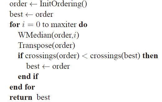
To solve this ILP, Graphviz employs a network simplex formulation [3]. Having obtained a ranking for the vertices of the graph, we turn to the ordering of vertices within each rank. The ordering of these vertices determines the number of edge crossings in the drawing, so our goal is to compute an ordering with the minimum number of crossings. Unfortunately, solving this problem exactly is NP-complete, so heuristic methods are employed. Computation of a good vertex ordering is an iterative process, with initial ordering computed by depth or breadth-first search starting at the vertices of minimum rank. Vertices are assigned positions within their ranks in left-to-right order as the search progresses.

为了解决这个 ILP，Graphviz 采用了网络单纯形公式 [3]。在为图的顶点获得排名后，我们转向每个排名内的顶点排序。这些顶点的排序决定了绘图中边交叉的数量，因此我们的目标是计算出具有最少交叉的排序。不幸的是，精确解决这个问题是 NP 完全的，因此采用启发式方法。计算一个好的顶点排序是一个迭代过程，初始排序通过从最低排名的顶点开始的深度优先搜索或广度优先搜索来计算。随着搜索的进行，顶点在其排名内从左到右分配位置。

Algorithm 2 Ordering()
算法 2：排序（Ordering）

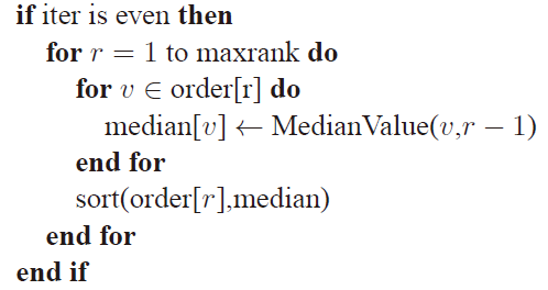
The weighted median heuristic assigns each vertex a median based on the positions of the adjacent vertices in the previous rank. The median value of a vertex is defined as the median position of its adjacent vertices if that value is uniquely defined. If such a value is not defined, the median is interpolated. The weighted median heuristic biases the median value to the side where vertices are more closely packed. Finally, the vertices are sorted within their rank by their assigned median values.

加权中位数启发式方法根据前一排名中相邻顶点的位置为每个顶点分配一个中位数。如果该值唯一确定，则顶点的中位数值定义为其相邻顶点的中位数位置。如果未定义该值，则通过插值计算中位数。加权中位数启发式方法将中位数值偏向顶点更密集的一侧。最后，根据分配的中位数值对顶点在其排名内进行排序。

Algorithm 3 WMedian(order,iter)

算法 3：加权中位数（WMedian）

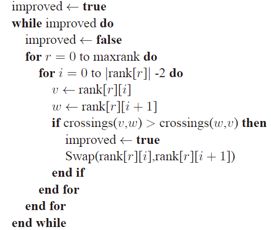
The transpose operation iterates through each rank examining neighboring vertices within a rank. Two vertices are swapped if swapping them decreases the number of edge crossings in the layout. The transpose operation terminates when no swap operation will further decrease the number of crossings. Since a minimum must exist, termination is guaranteed. Once a good ordering is found within each rank, all that remains is to assign $x$ and $y$ coordinates to each vertex and create the splines to draw the edges. The $y$ coordinates are based on the rank, so vertices with the same rank will appear on the same level. The $x$ coordinates are determined using the ordering and chosen to keep the edges short. Finally, splines are computed for each edge.

转置操作遍历每个等级，检查等级内的相邻顶点。如果交换两个顶点可以减少布局中的边交叉数量，则交换它们。当没有交换操作可以进一步减少交叉数量时，转置操作终止。由于存在最小值，因此可以保证终止。在每个等级内找到一个好的排序后，剩下的就是为每个顶点分配 $x$ 和 $y$ 坐标，并为绘制边计算样条曲线。$y$ 坐标基于等级，因此具有相同等级的顶点将出现在同一水平线上。$x$ 坐标根据排序确定，选择的目的是使边尽可能短。最后，为每条边计算样条曲线。

Algorithm 4 Transpose(rank)

算法 4：转置（Transpose）

6 Conclusion

结论
Graphviz is an extremely powerful and widely used tool for visualizing graphs. Several algorithms have been presented above for drawing the most common types of graphs. For small unweighted undirected graphs, fdp or neato will produce a good drawing. Once these graphs exceed 10000 vertices sfdp should be used. Unfortunately, sfdp does not take edge weights into account. To draw large weighted undirected graphs, low-rank stress majorization must be employed. Finally, dot is the tool of choice for visualization of directed graphs and trees.
Graphviz 是一个功能极其强大且被广泛使用的图可视化工具。上文介绍了几种用于绘制最常见类型图的算法。对于小型无权无向图，fdp 或 neato 可以生成良好的绘制效果。当这些图的顶点数超过 10000 时，应使用 sfdp。遗憾的是，sfdp 不考虑边的权重。要绘制大型加权无向图，必须采用低秩应力主化方法。最后，对于有向图和树的可视化，dot 是首选工具。

7 Acknowledgements

致谢

I would like to thank my reviewer, Michael Schoenberg, whose helpful comments drastically improved this manuscript.

我要感谢我的审稿人 Michael Schoenberg，他的有益建议极大地改进了本文。

A Laplacian Matrices

A. 拉普拉斯矩阵

The Laplacian matrix of a graph $G$ is a representation of $G$ similar to the adjacency matrix. In fact, the Laplacian matrix can be defined in terms of the degree matrix and the adjacency matrix. As we proceed, consider a simple graph $G$ with $n=|V|$ and $m=|E|$.

图 $G$ 的拉普拉斯矩阵是 $G$ 的一种表示，类似于邻接矩阵。实际上，拉普拉斯矩阵可以用度矩阵和邻接矩阵来定义。在继续之前，考虑一个简单图 $G$，其中 $n=|V|$ 和 $m=|E|$。

Definition 3 The adjacency matrix $A$ for a graph $G$ is the $n\times n$ matrix given by:

定义 3：图 $G$ 的邻接矩阵 $A$ 是一个 $n\times n$ 矩阵，定义为：

$$A_{i,j}=\{\begin{array}{ll}1& \text{if }(i,j)\in E\\ 0& \text{otherwise}\end{array}$$

Definition 4 The Laplacian matrix $L$ for an unweighted, undirected graph $G$ is the $n\times n$ matrix given by:

定义 4：无权无向图 $G$ 的拉普拉斯矩阵 $L$ 是一个 $n\times n$ 矩阵，定义为：

$$L_{i,j}=\{\begin{array}{ll}\mathrm{deg}(i)& \text{if }i=j\\ -1& \text{if }(i,j)\in E\\ 0& \text{otherwise}\end{array}$$

where $\mathrm{deg}(i)$ is the degree of the $i$-th vertex.

其中 $\mathrm{deg}(i)$ 是第 $i$ 个顶点的度。

For each edge $(i,j)\in E$ the entry $L_{i,j}=-1$. Additionally, the degrees of each vertex are stored on the diagonal elements. The Laplacian matrix can also be expressed as

对于每条边 $(i,j)\in E$，矩阵条目 $L_{i,j}=-1$。此外，每个顶点的度存储在对角线元素中。拉普拉斯矩阵也可以表示为

$$L=D-A$$

where $D$ is the degree matrix and $A$ is the adjacency matrix.

其中 $D$ 是度矩阵，$A$ 是邻接矩阵。

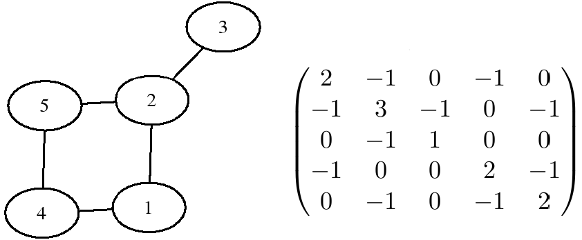
Figure 10: A simple graph and its Laplacian matrix
图 10：一个简单图及其拉普拉斯矩阵

All Laplacian matrices are positive-semidefinite and, as a result, have all nonnegative eigenvalues, $\forall i{\lambda }_i\ge 0$. The number of times that 0 appears as an eigenvalue is equal to the number of connected components in the graph. Thus ${\lambda }_0=0$ for any Laplacian matrix. The first eigenvector ${\mathbf{v}}_0$, corresponding to the eigenvalue ${\lambda }_0$, is always equal to $1=(1,1,\dots ,1)\in {\mathbb{R}}^n$. Notice that $L{\mathbf{v}}_0=0$ because the sum of the elements in any row is 0. The null space of a Laplacian matrix is always nontrivial, but if $G$ is a connected graph then the null space is a 1D subspace spanned by the vector $1$. In general, the dimension of the null space is equal to the number of connected components in $G$.

所有拉普拉斯矩阵都是半正定的，因此其所有特征值均为非负，$\forall i{\lambda }_i\ge 0$。0 作为特征值出现的次数等于图中连通分量的数量。因此，对于任何拉普拉斯矩阵，${\lambda }_0=0$。第一个特征向量 ${\mathbf{v}}_0$，对应于特征值 ${\lambda }_0$，总是等于 $1=(1,1,\dots ,1)\in {\mathbb{R}}^n$。注意，$L{\mathbf{v}}_0=0$，因为任何一行的元素之和为 0。拉普拉斯矩阵的零空间总是非平凡的，但如果 $G$ 是连通图，则零空间是一个由向量 $1$ 张成的 1 维子空间。一般来说，零空间的维度等于 $G$ 中连通分量的数量。

References

参考文献

[1] AT&T Labs. http://www.graphviz.org/Documentation.php.

[2] J. Barnes and P. Hut. A hierarchical O(N log N) force-calculation algorithm. Nature, 324(6096):446– 449, Dec. 1986.

[3] V. Chvatal. Linear Programming. W. H. Freeman, 1st edition, 1983.

[4] T. H. Cormen, C. E. Leiserson, R. L. Rivest, and C. Stein. Introduction to Algorithms. The MIT Press, 3rd edition, 2009.

[5] E. Gansner, Y. Koren, and S. North. Graph drawing by stress majorization. In J. Pach, editor, Graph Drawing, volume 3383 of Lecture Notes in Computer Science, pages 239–250. Springer Berlin / Heidelberg, 2005.

[6] E. R. Gansner, E. Koutsofios, S. C. North, and K. phong Vo. A technique for drawing directed graphs. IEEE Transactions on Software Engineering, 19(3):214–230, 1993.

[7] Y. F. Hu. Efficient and high quality force-directed graph drawing. The Mathematica Journal, 10:37–71, 2005.

[8] M. Khoury, Y. Hu, S. Krishnan, and C. Scheidegger. Drawing large graphs by low-rank stress majorization. Computer Graphics Forum, To Appear.

[9] J. R. Shewchuk. An introduction to the conjugate gradient method without the agonizing pain. Technical report, Carnegie Mellon University, Pittsburgh, PA, USA, 1994.

---

篇外：排障讨论

注：机翻，未校。

“RuntimeError: Make sure the Graphviz executables are on your system’s path” after installing Graphviz 2.38

I downloaded Graphviz 2.38 MSI version and installed under folder C:\Python34, then I run pip install Graphviz, everything went well. In system’s path I added C:\Python34\bin. When I tried to run a test script, in line filename=dot.render(filename='test'), I got a message

我下载了 Graphviz 2.38 MSI 版本并安装在文件夹 C:\Python34 下，然后运行 pip install Graphviz，一切顺利。我在系统的路径中添加了 C:\Python34\bin。当我尝试运行一个测试脚本时，在 filename=dot.render(filename='test') 这一行，我收到了一条消息：

RuntimeError: failed to execute [‘dot’, ‘-Tpdf’, ‘-O’, ‘test’], make sure the Graphviz executables are on your systems’ path

I tried to put "C:\Python34\bin\dot.exe" in system’s path, but it didn’t work, and I even created a new environment variable "GRAPHVIZ_DOT" with value "C:\Python34\bin\dot.exe", still not working. I tried to uninstall Graphviz and pip uninstall graphviz, then reinstall it and pip install again, but nothing works.

我尝试将 "C:\Python34\bin\dot.exe" 添加到系统的路径中，但不起作用，我还创建了一个新的环境变量 "GRAPHVIZ_DOT"，值为 "C:\Python34\bin\dot.exe"，但仍然不起作用。我尝试卸载 Graphviz 并运行 pip uninstall graphviz，然后重新安装并再次使用 pip 安装，但仍然没有解决问题。

The whole traceback message is:

完整的回溯信息如下：

```python
Traceback (most recent call last):
File “C:\Python34\lib\site-packages\graphviz\files.py”, line 220, in render
proc = subprocess.Popen(cmd, startupinfo=STARTUPINFO)
File “C:\Python34\lib\subprocess.py”, line 859, in init
restore_signals, start_new_session)
File “C:\Python34\lib\subprocess.py”, line 1112, in _execute_child
startupinfo)
FileNotFoundError: [WinError 2] The system cannot find the file specified
During handling of the above exception, another exception occurred:
Traceback (most recent call last):
File “C:\Users\Documents\Kissmetrics\curves and lines\eventNodes.py”, line 56, in
filename=dot.render(filename=‘test’)
File “C:\Python34\lib\site-packages\graphviz\files.py”, line 225, in render
‘are on your systems’ path’ % cmd)
RuntimeError: failed to execute [‘dot’, ‘-Tpdf’, ‘-O’, ‘test’], make sure the Graphviz executables are on your systems’ path
```

Does anybody have any experience with it?

有人遇到过类似的问题吗？

edited Dec 24, 2019 at 14:59 UserAG
asked Jan 28, 2016 at 14:35 liga810

Answers

You should install the graphviz package in your system (not just the python package). On Ubuntu you should try:

你应该在系统中安装 Graphviz 软件包（而不仅仅是 Python 包）。在 Ubuntu 上，你可以尝试：

sudo apt-get install graphviz

edited Mar 8, 2018 at 15:23 Sainath Adapa
answered Mar 18, 2017 at 14:13 kame

If this doesn’t work (it says the package is referenced but not there or something like that) run sudo apt-get update in order to update apt-get and tell it what packages are there.

如果不起作用（它提示包被引用但不存在，或者其他类似的错误），运行 sudo apt-get update 来更新 apt-get，并告知它有哪些包可用。

– Pro Q

Commented Jan 21, 2018 at 0:39

If you’re in a Docker Container (like I was), I was already at root and only needed apt-get install graphviz

如果你在 Docker 容器中（就像我一样），我已经处于 root 用户，只需要运行 apt-get install graphviz。

– kevin_theinfinityfund

Commented Jun 15, 2020 at 17:00

Hope I can help someone with this. It did not work the first time for me so I ran sudo apt-get update && sudo apt-get upgrade and it worked afterwards.

希望我的经验能帮到别人。第一次我没有成功，所以我运行了 sudo apt-get update && sudo apt-get upgrade，之后就成功了。

– dylanvanw

Commented Apr 15, 2021 at 11:15

What if I just want to install graphviz in a virtual environment?

如果我只是想在虚拟环境中安装 Graphviz，该怎么办？

– Vadim

Commented May 26, 2023 at 17:59

This one should solve the problem on MacOS:

这个方法应该可以解决在 MacOS 上的问题：

brew install graphviz

To explain the misconception for new comer who using Conda. When we run conda install graphviz, it install the binary of Graphviz (this is not executable in Python yet).

解释一下对于使用 Conda 的新手来说可能存在的误解。当我们运行 conda install graphviz 时，它安装的是 Graphviz 的二进制文件（这在 Python 中还不可执行）。

And then we usually will also install conda install python-graphviz, this install the wrapper for python to run the binary of graphviz, the problem is we might get errors with message “graphviz” not executeable.

然后我们通常还会安装 conda install python-graphviz，它安装了用于 Python 的 Graphviz 二进制文件的包装器，但问题是我们可能会收到错误消息，提示 “graphviz” 不可执行。

Thus why better use homebrew to install Graphviz binary and then install python-graphviz. Homebrew will guarantee the binary executable.

因此，建议使用 Homebrew 安装 Graphviz 的二进制文件，然后再安装 python-graphviz。Homebrew 可以保证二进制文件的可执行性。

edited Aug 23, 2024 at 7:21 Astariul

answered Jul 30, 2016 at 2:46 Rouzbeh

For mac, it seem this is best option. Unless you want to use MacPorts and install graphviz from here: Download.

对于 Mac，这似乎是最好的选择。除非你想使用 MacPorts 并从这里安装 Graphviz：Download

– Alex

Commented Nov 25, 2016 at 19:14

How do I find my bin folder where I have graphviz. I am having this problem and is really killing right now. Just checked I have graphviz 2.38.

我该如何找到安装了 Graphviz 的 bin 文件夹？我现在遇到了这个问题，非常困扰。我刚刚检查了，我安装的是 Graphviz 2.38。

– Herc01

Commented Feb 21, 2019 at 16:05

Before brew install graphviz worked I had to run: xcode-select --install

在运行 brew install graphviz 之前，我还需要运行：xcode-select --install。

– Va5ili5

Commented Feb 2, 2022 at 13:59

Thank you. I installed graphviz with pip but only worked when I installed it with homebrew.

谢谢。我通过 pip 安装了 Graphviz，但只有通过 homebrew 安装后才起作用。

– Leonardo

Commented Apr 10, 2022 at 12:56

No brew does not.

不，brew 并没有。

– sajid

Commented Aug 18, 2022 at 8:17

import os
os.environ["PATH"] += os.pathsep + 'D:/Program Files (x86)/Graphviz2.38/bin/'

In windows just add these 2 lines in the beginning, where ‘D:/Program Files (x86)/Graphviz2.38/bin/’ is replaced by the address of where your bin file is.

在 Windows 中，只需在开头添加这两行代码，其中 ‘D:/Program Files (x86)/Graphviz2.38/bin/’ 替换为你的 bin 文件的路径。

That solves the problem.

这可以解决这个问题。

answered Jun 19, 2017 at 8:43

Aprameyo Roy

worked in windows, I downloaded graphviz-2.38.zip from here Download.

在 Windows 中有效，我从这里下载了 graphviz-2.38.zip：Download

– user3046442

Commented Mar 14, 2018 at 8:15

This works for me. I tried to add this to user and system environment variables, but that doesn’t work, only your solution works for me.

这个方法对我有效。我尝试将其添加到用户和系统的环境变量中，但不起作用，只有你的解决方案对我有效。

– Tom

Commented Oct 25, 2018 at 17:05

this worked for me as well, but it threw another error before working. For some reason It gave me a side-by-side configuration…-error. I had to additionally reinstall the Microsoft Visual C++ 2008 Redistributable Package (x86). If someone has the same problem, here’s the link: microsoft.com/de-DE/download/details.aspx?id=29

这个方法对我也有效，但在起作用之前它还抛出了另一个错误。不知为何，它提示了一个并行配置错误……我不得不重新安装了 Microsoft Visual C++ 2008 Redistributable Package (x86)。如果有人遇到同样的问题，这里有一个链接：microsoft.com/de-DE/download/details.aspx?id=29

– Marco

Commented Dec 29, 2018 at 8:00

I used chocolatey to install graphviz choco install -y graphviz

我使用 chocolatey 安装了 Graphviz：choco install -y graphviz

– reddi.tech

Commented Mar 20, 2020 at 9:06

Yep this worked. make sure to download the right graphviz. I also placed the graphviz bins on both user and system paths.

这个方法有效。确保下载了正确的 Graphviz。我还把 Graphviz 的 bin 文件夹添加到了用户和系统的路径中。

– max

Commented Oct 7, 2020 at 22:03

For Windows:

1. Install windows package from: Download
   从 Download 下载 Windows 安装包

2. Install python graphviz package
   安装 Python 的 graphviz 包

3. Add C:\Program Files (x86)\Graphviz2.38\bin to User path
   将 C:\Program Files (x86)\Graphviz2.38\bin 添加到用户路径中

4. Add C:\Program Files (x86)\Graphviz2.38\bin\dot.exe to System Path
   将 C:\Program Files (x86)\Graphviz2.38\bin\dot.exe 添加到系统路径中

This worked for me!

这个方法对我有效！

edited Jul 9, 2018 at 20:14
answered May 16, 2017 at 15:05 Jyotsna_b

Also Close your “cmd” in which jupyter notebook is running. Existing running CMD dont catch the new changes in Environment variables.

另外，关闭正在运行 Jupyter Notebook 的命令提示符窗口。正在运行的 CMD 窗口无法捕获环境变量中的新更改。

– Rohit Nandi

Commented Apr 15, 2018 at 8:46

It didn’t work for me until I restarted the system

直到我重启系统后，这个方法才有效。

– Mohammad Nazari

Commented Dec 4, 2019 at 0:31

This worked perfectly. Just had to restart the notebook again. Thanks.

这个方法完美有效。只需要重新启动 Jupyter Notebook 即可。谢谢。

– Amresh Giri

Commented Apr 20, 2020 at 7:55

You don’t need to restart the entire system, but just the python kernel.

你不需要重启整个系统，只需要重启 Python 内核。

– SujaiSparks

Commented Jul 21, 2022 at 10:04

2

@SujaiSparks - didn’t work - I had to restart the entire system.

@SujaiSparks - 不起作用，我不得不重启整个系统。

– Alaa M.

Commented Jan 29, 2023 at 19:27

Try using:
尝试使用：

conda install python-graphviz

The graphviz executable sit on a different path from your conda directory, if you use pip install graphviz.

如果你使用 pip install graphviz，Graphviz 的可执行文件路径将与你的 conda 目录不同。

edited Nov 3, 2018 at 23:51

answered Oct 29, 2018 at 9:00 Abishek

4

Conda install graphviz worked on windows! nothing else seems to work :\

在 Windows 上，Conda install graphviz 起作用了！其他方法似乎都不行。

– Joel Carneiro

Commented Jan 29, 2019 at 15:00

pygraphviz have a nice big warning against using conda, Not clear why, though.

pygraphviz 有一个 明显的警告，反对使用 conda，但不清楚原因。

– Adam Burke

Commented Feb 24, 2021 at 6:07

I ran conda install python-graphviz in my Anaconda prompt and once the execution is done, just restart the Jupyter notebook kernel. It worked for me.

我在 Anaconda 提示符中运行了 conda install python-graphviz，执行完成后，只需重新启动 Jupyter Notebook 内核即可。这个方法对我有效。

– mpriya

Commented Mar 3, 2021 at 7:52

I ran conda install python-graphviz in my Anaconda prompt and once the execution is done, just restart the Jupyter notebook kernel. It worked for me. Worked on Windows as well.

我在 Anaconda 提示符中运行了 conda install python-graphviz，执行完成后，只需重新启动 Jupyter Notebook 内核即可。这个方法对我有效。在 Windows 上也有效。

– Mata

Commented May 19, 2023 at 14:0129

Step 1: Install Graphviz binary

安装 Graphviz 二进制文件

Windows:

1. Download Graphviz from Download

2. Add below to PATH environment variable (mention the installed graphviz version):

   将以下路径添加到 PATH 环境变量中（指定安装的 Graphviz 版本）：

   • C:\Program Files (x86)\Graphviz2.38\bin
   • C:\Program Files (x86)\Graphviz2.38\bin\dot.exe

3. Close any opened Juypter notebook and the command prompt

   关闭所有打开的 Jupyter Notebook 和命令提示符

4. Restart Jupyter / cmd prompt and test

   重新启动 Jupyter 或命令提示符并进行测试

Linux:

1. sudo apt-get update
   

2. sudo apt-get install graphviz
   

3. or build it manually from Download

Step 2: Install graphviz module for python

安装 Python 的 graphviz 模块

pip:

pip install graphviz

conda:

conda install graphviz

answered May 19, 2019 at 2:58

Chankey Pathak

Solved for me on winzoz

– rakwaht

Commented Jun 14, 2019 at 11:40

Others also answered the question, but this “takes you by the hand”. 🌟

– Ghulam

Commented Dec 27, 2023 at 15:34

---

via:

• windows 下 Graphviz 安装及入门教程 - CSDN 博客
  https://blog.csdn.net/lanchunhui/article/details/49472949

• [Graphviz 安装向导及入门指南 - CSDN 博客
  https://blog.csdn.net/m0_51143578/article/details/128434990

• GraphViz 使用教程-用代码生成有向图。并介绍流程图、时序图等绘图工具_graphviz使用教程-CSDN博客
  https://blog.csdn.net/youwen21/article/details/98896703

  • GraphViz 官方文档 - Documentation | Graphviz
    https://www.graphviz.org/documentation/

  • GraphViz 案例教程
    https://renenyffenegger.ch/notes/tools/Graphviz/examples/index

  • 类似 Graphviz 的工具是如何实现自动排版的
    https://www.zhihu.com/question/32098665

• Let’s Draw a Graph: an Introduction with Graphviz - DocsLib
  https://docslib.org/doc/8539071/lets-draw-a-graph-an-introduction-with-graphviz

• 程序员必知的图形工具
  https://mp.weixin.qq.com/s/YaEMA9gw2Uz9IdZIl0UAHw
  Graphviz的使用指南-CSDN博客
  https://blog.csdn.net/a6661314/article/details/122656342

• python - “RuntimeError: Make sure the Graphviz executables are on your system’s path” after installing Graphviz 2.38 - Stack Overflow
  https://stackoverflow.com/questions/35064304/runtimeerror-make-sure-the-graphviz-executables-are-on-your-systems-path-aft