opencv21:Histograms直方图-查找、绘制和分析

目标

学会

• 使用OpenCV和Numpy函数查找直方图
• 使用OpenCV和Matplotlib函数绘制直方图
• 函数：cv2.calcHist()，np.histogram()等。

理论

直方图(Histograms)是什么？可以将直方图视为图形或绘图，从而可以总体了解图像的强度分布。它是在X轴上具有像素值（不总是从0到255的范围），在Y轴上具有图像中相应像素数量的图。

hog只是理解图像的另一种方式。通过查看图像的直方图，可以直观地了解该图像的对比度，亮度，强度分布等。当今几乎所有图像处理工具都提供直方图功能。下图来自网站（ Cambridge in Color website）的图片

可以看到图像及其直方图。（记住，直方图是针对灰度图像而非彩色图像绘制的）。直方图的左侧区域显示图像中较暗像素的数量，而右侧区域则显示明亮像素的数量。从直方图中，可以看到暗区域多于亮区域，而中间调的数量（中间值的像素值，例如127附近）则非常少。

寻找直方图

现在有了关于直方图的认识，就可以研究如何找到它。OpenCV和Numpy都为此内置了实现函数。在使用这些函数之前，需要了解一些与直方图有关的术语。

• BINS：上面的直方图显示每个像素值的像素数，即从0到255。即，需要256个值来显示上面的直方图。但是假设如果不需要分别找到所有像素值的像素数，而是找到像素值间隔中的像素数怎么办？
  例如，需要找到介于0到15之间的像素数，然后找到16到31之间，…，240到255之间的像素数。只需要16个值即可表示直方图。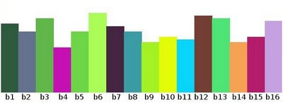
  因此，要做的就是将整个直方图分成16个子部分，每个子部分的值就是其中所有像素数的总和。
  每个子部分都称为BIN。在第一种情况下，bin的数量为256个（每个像素一个），而在第二种情况下，bin的数量仅为16个。BINS由OpenCV文档中的histSize术语表示。

• DIMS：为其收集数据的参数的数量。在这种情况下，仅收集关于强度值这一件事的数据，所以这里是1。

• RANGE：要测量的强度值的范围。通常，它是[0,256]，即所有强度值。

OpenCV中的直方图计算

在OpenCv中，可以使用cv2.calcHist()函数查找直方图。熟悉一下该函数及其参数：

cv2.calcHist（images，channels，mask，histSize，ranges [，hist [，accumulate]]）

• images：它是uint8或float32类型的源图像。它应该放在方括号中，即 [img]
• channels：也以方括号给出。是计算直方图的通道的索引。例如，如果输入为灰度图像，则其值为[0]。对于彩色图像，可以传递[0]，[1]或[2]分别计算蓝色，绿色或红色通道的直方图
• mask：图像掩码。为了找到完整图像的直方图，将其指定为“无”。但是，如果要查找图像特定区域的直方图，则必须为此创建一个掩码图像并将其作为掩码
• histSize：这表示BIN计数。需要放在方括号中。对于全尺寸，设置为[256]
• ranges：这是RANGE。通常为[0,256]
  

img = cv.imread('home.jpg',0)
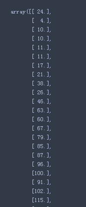
hist = cv.calcHist([img],[0],None,[256],[0,256]) 

hist是256x1的数组，每个值对应于该图像中具有相应像素值的像素数

Numpy的直方图计算

Numpy也提供了一个函数np.histogram()。因此，除了cv2.calcHist()函数外，可以尝试下面的代码：

import numpy as np
hist, bins = np.histogram(img.ravel(), 256, [0,256])   # 先展成一维再统计

可以看到，hist与opencv计算的结果相同。但是bin具有257个元素(0~256)，因为Numpy计算出bin的范围为0-0.99、1-1.99、2-2.99等, 因此最终范围为255-255.99。为了表示这一点，他们还在最后添加了256。但使用时候不需要256， 最多255就足够了。

另外
Numpy还有另一个函数np.bincount()，它比np.histogram()快10倍左右。因此，对于一维直方图，可以更好地尝试一下。不要忘记在np.bincount中设置minlength = 256。例如，

hist = np.bincount(img.ravel()，minlength = 256)  # 先展成一维再统计

注意
OpenCV函数cv2.calcHist()比np.histogram()快大约40倍。因此，尽可能使用OpenCV函数的cv2.calcHist()。

绘制直方图

绘制直方图有两种方法，

• 简短的方法：使用Matplotlib绘图功能
• 稍长的方法：使用OpenCV绘图功能

使用Matplotlib

Matplotlib带有直方图绘图功能：matplotlib.pyplot.hist()
它直接找到直方图并将其绘制, 无需使用calcHist()或np.histogram()函数来查找直方图。代码如下：

import cv2
import numpy as np
from matplotlib import pyplot as plt
img = cv2.imread('hog.jpg', 0)
plt.subplot(1,2,1)
plt.imshow(img, cmap='gray')
plt.subplot(1,2,2)
plt.hist(img.ravel(), 256, [0,256])
plt.show()

结果如下：

或者，可以使用matplotlib的法线图，这对于BGR图是很好的。为此，需要首先找到直方图数据。代码如下：

import numpy as np
import cv2 as cv
from matplotlib import pyplot as plt
img = cv.imread('hog.jpg')
color = ('b','g','r')
for i,col in enumerate(color):
    histr = cv.calcHist([img],[i],None,[256],[0,256])
    plt.plot(histr,color = col)
    plt.xlim([0,256])
plt.show()

结果如下：

可以从上图中得出，蓝色在图像中具有一些高值域（显然这应该是由于天空）

使用 OpenCV

在这里可以调整直方图的值及其bin值，使其看起来像x，y坐标，以便可以使用cv2.line()或cv2.polyline()函数绘制它以生成与上述相同的图像。OpenCV-Python官方示例已经提供了样例代码

#!/usr/bin/env python
# https://github.com/opencv/opencv/blob/master/samples/python/hist.py
''' This is a sample for histogram plotting for RGB images and grayscale images for better understanding of colour distribution

Benefit : Learn how to draw histogram of images
          Get familier with cv.calcHist, cv.equalizeHist,cv.normalize and some drawing functions

Level : Beginner or Intermediate

Functions : 1) hist_curve : returns histogram of an image drawn as curves
            2) hist_lines : return histogram of an image drawn as bins ( only for grayscale images )

Usage : python hist.py <image_file>

Abid Rahman 3/14/12 debug Gary Bradski
'''

# Python 2/3 compatibility
from __future__ import print_function

import numpy as np
import cv2 as cv

bins = np.arange(256).reshape(256,1)

def hist_curve(im):
    h = np.zeros((300,256,3))
    if len(im.shape) == 2:
        color = [(255,255,255)]
    elif im.shape[2] == 3:
        color = [ (255,0,0),(0,255,0),(0,0,255) ]
    for ch, col in enumerate(color):
        hist_item = cv.calcHist([im],[ch],None,[256],[0,256])
        cv.normalize(hist_item,hist_item,0,255,cv.NORM_MINMAX)
        hist=np.int32(np.around(hist_item))
        pts = np.int32(np.column_stack((bins,hist)))
        cv.polylines(h,[pts],False,col)
    y=np.flipud(h)
    return y

def hist_lines(im):
    h = np.zeros((300,256,3))
    if len(im.shape)!=2:
        print("hist_lines applicable only for grayscale images")
        #print("so converting image to grayscale for representation"
        im = cv.cvtColor(im,cv.COLOR_BGR2GRAY)
    hist_item = cv.calcHist([im],[0],None,[256],[0,256])
    cv.normalize(hist_item,hist_item,0,255,cv.NORM_MINMAX)
    hist = np.int32(np.around(hist_item))
    for x,y in enumerate(hist):
        cv.line(h,(x,0),(x,y[0]),(255,255,255))
    y = np.flipud(h)
    return y


def main():
    import sys

    if len(sys.argv)>1:
        fname = sys.argv[1]
    else :
        fname = 'lena.jpg'
        print("usage : python hist.py <image_file>")

    im = cv.imread(cv.samples.findFile(fname))

    if im is None:
        print('Failed to load image file:', fname)
        sys.exit(1)

    gray = cv.cvtColor(im,cv.COLOR_BGR2GRAY)


    print(''' Histogram plotting \n
    Keymap :\n
    a - show histogram for color image in curve mode \n
    b - show histogram in bin mode \n
    c - show equalized histogram (always in bin mode) \n
    d - show histogram for gray image in curve mode \n
    e - show histogram for a normalized image in curve mode \n
    Esc - exit \n
    ''')

    cv.imshow('image',im)
    while True:
        k = cv.waitKey(0)
        if k == ord('a'):
            curve = hist_curve(im)
            cv.imshow('histogram',curve)
            cv.imshow('image',im)
            print('a')
        elif k == ord('b'):
            print('b')
            lines = hist_lines(im)
            cv.imshow('histogram',lines)
            cv.imshow('image',gray)
        elif k == ord('c'):
            print('c')
            equ = cv.equalizeHist(gray)
            lines = hist_lines(equ)
            cv.imshow('histogram',lines)
            cv.imshow('image',equ)
        elif k == ord('d'):
            print('d')
            curve = hist_curve(gray)
            cv.imshow('histogram',curve)
            cv.imshow('image',gray)
        elif k == ord('e'):
            print('e')
            norm = cv.normalize(gray, gray, alpha = 0,beta = 255,norm_type = cv.NORM_MINMAX)
            lines = hist_lines(norm)
            cv.imshow('histogram',lines)
            cv.imshow('image',norm)
        elif k == 27:
            print('ESC')
            cv.destroyAllWindows()
            break

    print('Done')


if __name__ == '__main__':
    print(__doc__)
    main()
    cv.destroyAllWindows()

掩码的应用

使用cv2.calcHist()能查找整个图像的直方图。如果想找到图像某些区域的直方图呢?只需创建一个掩码图像，将要找到直方图为白色，否则黑色， 然后把这个作为掩码传递。

import numpy as np
import cv2 as cv
from matplotlib import pyplot as plt

img = cv2.imread('hog.jpg', 0)
# create a mask
mask = np.zeros(img.shape[:2], np.uint8)
mask[100:200, 100:200] = 255  # set white
masked_img = cv2.bitwise_and(img,img,mask = mask)
# Calculate histogram with mask and without mask
# Check third argument for mask
hist_full = cv2.calcHist([img], [0], None, [256],[0,256])
hist_mask = cv2.calcHist([img], [0], mask, [256], [0,256])

# plt.subplot(221) <--> plt.subplot(2,2,1)
plt.subplot(2,2,1)
plt.imshow(img, cmap='gray')
plt.subplot(2,2,2)
plt.imshow(mask, cmap='gray')
plt.subplot(2,2,3)
plt.imshow(masked_img, cmap='gray')
plt.subplot(2, 2, 4)
plt.plot(hist_full, color='r')
plt.plot(hist_mask, color='g')
plt.xlim([0, 255])
plt.show()
plt.show()

查看结果。在直方图中，蓝线表示完整图像的直方图，绿线表示掩码区域的直方图。

附加资源

• https://docs.opencv.org/4.1.2/d1/db7/tutorial_py_histogram_begins.html
• Cambridge in Color website
• https://docs.opencv.org/4.1.2/d8/dbc/tutorial_histogram_calculation.html
• https://github.com/opencv/opencv/blob/master/samples/python/hist.py
• https://zhuanlan.zhihu.com/p/36656952