稀疏矩阵之scipy

稀疏矩阵

矩阵中包含少量的非零项，则称之为稀疏矩阵。

对于稀疏矩阵，它通常具有很大的维度，有时甚大到整个矩阵（零元素）占用了绝大部分内存。

采用二维数组的存储方法既浪费大量的存储单元来存放零元素，又要在运算中浪费大量的时间来进行零元素的无效运算。因此必须考虑对稀疏矩阵进行压缩存储（只存储非零元素）。

稀疏矩阵可以通过scipy.sparse来构造。

常用的矩阵形式：

1. coo_matrix((data, (i, j)), [shape=(M, N)])
2. csc_matrix((data, indices, indptr), [shape=(M, N)])：逐行压缩矩阵
3. csr_matrix((data, indices, indptr), [shape=(M, N))：逐列压缩矩阵

矩阵属性

公共属性：

• mat.shape ： 矩阵形状
• mat.dtype ： 数据类型
• mat.ndim ： 矩阵维度
• mat.nnz ： 非零个数
• mat.data ： 非零值, 一维数组

coo_matrix矩阵形式：

• coo.row ： 矩阵行索引
• coo.col ： 矩阵列索引

csc_matrix\csr_matrix 形式：

• csc_matrix.indices ： 索引数组
• csc_matrix.indptr ： 指针数组
• csc_matrix.has_sorted_indices ： 索引是否排序
• csc_matrix.blocksize ： 矩阵块大小

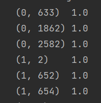
coo_matrix矩阵形式

>>> # Constructing a matrix using ijv format
>>> row  = np.array([0, 3, 1, 0])
>>> col  = np.array([0, 3, 1, 2])
>>> data = np.array([4, 5, 7, 9])
>>> coo_matrix((data, (row, col)), shape=(4, 4)).toarray()
array([[4, 0, 9, 0],
       [0, 7, 0, 0],
       [0, 0, 0, 0],
       [0, 0, 0, 5]])

经常的用法大概是这样的：coo_matrix((data, (i, j)), [shape=(M, N)])

这里有三个参数：

1. data[:] 就是原始矩阵中的数据，例如上面的4,5,7,9；

2. i[:] 就是行的指示符号；例如上面row的第0个元素是0，就代表data中第一个数据在第0行；

3. j[:] 就是列的指示符号；例如上面col的第0个元素是0，就代表data中第一个数据在第0列；

综合上面三点，对data中第一个数据4来说，就是原始矩阵中有4这个元素，它在第0行，第0列，即A[i[k], j[k]] = data[k]。以此类推，data中第2个数据5，在第3行，第3列。

最后，有个shape参数是告诉coo_matrix原始矩阵的形状，除了上述描述的有数据的行列，其他地方都按照shape的形式补0。

csr_matrix 矩阵形式

csr_matrix((data, indices, indptr), [shape=(M, N)])

• data数组表示存储的最终数据。
• 因为是csr的存储方式，indptr表示按行来”计算"。其中第i行的非零数据为data[indptr[i]:indptr[i+1]]。
• 而对应的非零数值的列索引存储在indices中，为indices[indptr[i]:indptr[i+1]]。

data = np.array([12,  2,  2,  2,  8, 12,  2,  2,  2,  2,  2,  2,  2,  8,  2,  2,  1, 1])
indices = np.array([1, 3, 5, 6, 7, 0, 3, 0, 1, 7, 0, 8, 0, 0, 4, 5, 9, 8])
indptr = np.array([ 0,  5,  7,  7,  9, 10, 12, 13, 15, 17, 18])

adj = sparse.csc_matrix((data, indices, indptr))
print(adj.toarray())
>> #输出
 [[ 0 12  0  2  0  2  2  8  0  0]
 [12  0  0  2  0  0  0  0  0  0]
 [ 0  0  0  0  0  0  0  0  0  0]
 [ 2  2  0  0  0  0  0  0  0  0]
 [ 0  0  0  0  0  0  0  2  0  0]
 [ 2  0  0  0  0  0  0  0  2  0]
 [ 2  0  0  0  0  0  0  0  0  0]
 [ 8  0  0  0  2  0  0  0  0  0]
 [ 0  0  0  0  0  2  0  0  0  1]
 [ 0  0  0  0  0  0  0  0  1  0]]

以第一行数据为例：
第一行的非零数据为：data[indptr[0]: indptr[1]]即data[0: 5]，即12, 2, 2, 2, 8，对应的列位置为indices[indptr[0]: indptr[1]]即1, 3, 5, 6, 7

所以最后的邻接矩阵：

adj[0][1]=12
adj[0][3]=2
adj[0][5]=2
adj[0][6]=2
adj[0][7]=8

表示

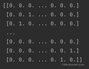
打印出这个矩阵adj时：

adj.todense()将返回adj矩阵的稠密表示：