有限元入门： 用变分法求解一维常微分方程(二)

承接上一篇博客
https://blog.csdn.net/waitingwinter/article/details/106164350
为了使结构完整，我们再次给出所求解的问题:
$$\{\begin{array}{rl}& -U^{\prime \prime }(t)+U(t)=({\pi }^2+1)\sin \pi t,\\ & U(0)=U(1)=0,\end{array}$$

二次有限元

数值格式

与之前有所不同的是, 我们取检验函数空间为 $V=H_0^2(\Omega )$,
将区间 [0,1] 等分为 N 个网格, 记 $t_i=i/N,$ 故有 $t_0=0,t_N=1.$ 令 $h_i=t_i-t_{i-1}$ 为网格尺寸. 因为等分网格, 故 $h_i=h=1/N,\forall i.$ 取基函数 ${\Phi }_i(i=2,3,\cdots ,N-2)$ 为分片二次函数.

引理：
对于分片多项式函数 $v$,$$v\in H^2(\Omega )\iff v\in C^1(\bar{\Omega }).$$
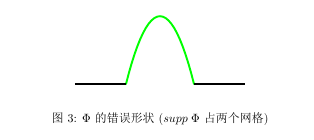
由上述引理知, 我们要构造整体 $C^1$ 的二次元, 故 $\Phi$ 不能为如下形式

$${\Phi }_i(t)=\{\begin{array}{rlr}& \frac{(t-t_{i-1}{)}^2}{h^2},& t\in (t_{i-1},t_i],\\ & \frac{(t_{i+1}-t{)}^2}{h^2},& t\in (t_i,t_{i+1}],\\ & 0,& otherwise.\end{array}$$
这里我采取了如下构造方式

$${\Phi }_i(t)=\{\begin{array}{rlr}& \frac{(t-t_{i-2}{)}^2}{2h^2},& t\in (t_{i-2},t_{i-1}],\\ & \frac{-(t_i-t{)}^2}{2h^2}+1,& t\in (t_{i-1},t_{i+1}],\\ & \frac{(t-t_{i+2}{)}^2}{2h^2},& t\in (t_{i+1},t_{i+2}],\\ & 0,& otherwise.\end{array}$$
令 $K_{ij}={\int }_0^1{\Phi }_i^{\prime }(t){\Phi }_j^{\prime }(t)+{\Phi }_i(t){\Phi }_j(t)dt,$ 经计算有
$$K_{ij}=\{\begin{array}{rlr}& \frac{4}{3h}+\frac{23}{15}h,& i=j,\\ & \frac{119h}{120}+\frac{1}{6h}& |i-j|=1,\\ & \frac{7h}{30}-\frac{2}{3h}& |i-j|=2,\\ & \frac{h}{120}-\frac{1}{6h}& |i-j|=3,\\ & 0,& otherwise.\end{array}$$
令 $$f_j={\int }_0^1({\pi }^2+1)\sin \pi t{\Phi }_j(t)\mathrm{d}t,$$
则有
$$f_j=\frac{4({\pi }^2+1)}{h^2{\pi }^3}(1-\cos h\pi )\sin h\pi \sin (\pi t_j),j=2,\cdots ,N-2.$$
记 $u=[u_2,u_3\cdots ,u_{N-2}{]}^T$, $F=[f_2,f_3,\cdots ,f_{N-2}{]}^T,$ 求解线性方程组
$$Ku=F,$$
注意到此矩阵为七对角矩阵, 用MATLAB求得方程的数值解 $$U_h(t)=\sum _{i=2}^{N-2}{u}_i{\Phi }_i(t).$$
解常微分方程, 容易求得问题的解为
$$U(t)=\sin \pi t.$$

需要注意的是，解出来的数值解是分片二次插值，所以严格来说，我的图中线性点与点线性插值是错误的.

误差估计

误差仍然采用之前的$$\Vert e\Vert ={\int }_{\Omega }|u^{\prime }(t)-u_h^{\prime }(t){|}^2\mathrm{d}t,$$
这个积分最好借助Mathematica来算（不太友好）。
数值实验结果如下图 所示, 使用 polyfit 拟合图像斜率有$$k=-0.9304,$$
即二次元的数值误差阶为 0.9304.

MATLAB代码

%% Quadratic function interpolation
err = zeros(8, 1);
n=10;
index = zeros(8,1);
for i=1:8
    index(i) = 2^(i-1) *n;
end
err_new = zeros(8,1);
for i = 1:8
    N = index(i);
    h = 1 / N;
    x = 0:h:1;
    xx = 0:1/1000:1;
    exact_solu = sin(pi.*xx);
    K = zeros(N-3);
    K = K + diag(ones(N-3,1).*(4/(3*h)+23/15*h), 0) + diag((119*h/120+1/(6*h)).*ones(N-4,1), 1) + diag((119*h/120+1/(6*h)).*ones(N-4,1), -1)+...
        diag((7*h/30-2/(3*h)).*ones(N-5,1), -2)+diag((7*h/30-2/(3*h)).*ones(N-5,1), 2)+diag((h/120-1/(6*h)).*ones(N-6,1), -3)+diag((h/120-1/(6*h)).*ones(N-6,1), 3);
    F = (pi^2+1)/(h^2*pi^3)*4*(1-cos(h*pi))*sin(pi*h)*sin(pi*x(3:N-1));
    K = sparse(K);
    coeff = K\F';
    solu = [0; 0; coeff; 0; 0] + 0.5.*[0; coeff; 0; 0; 0] + 0.5 * [0; 0; 0; coeff; 0];
    
    figure()
    plot(x', solu, '*--',xx', exact_solu, 'g--');
    legend('numerical solution', 'exact solution')
    xlabel('x')
    ylabel('U');
    %     ylim([0,1]);
    title(['numerical solution and exact solution N=',num2str(index(i))]);
    
    % calculate the error
    % 形式太复杂了, 尽管借助了mathematica， 但还是很不爽
    error  = 0;
    % 中间的 N-6块
    for j = 4 :1: (N-3)
        a = coeff(j);
        b = coeff(j-1);
        c = coeff(j-2);
        d = coeff(j-3);
        t = x(j);
        t_h = x(j+1);
        error = error + 1/(12*h^2*pi)*(24*(a-b-c+d)*(cos(pi*t)-cos(pi*(t_h)))+h*pi*...
            (4*a^2+4*a*b+4*b^2-8*a*c-4*b*c+4*c^2-4*a*d-8*b*d+4*c*d+4*d^2+6*h^2*pi^2+24*(b-d)*sin(pi*t)...
            +3*h*pi*(sin(2*pi*(t_h))-sin(2*pi*t))+24*(c-a)*sin(pi*(t_h))));
    end
    % 左边的3块
    a = coeff(1);
    b = coeff(2);
    c = coeff(3);
    error1 = 1/(6*h^2*pi)*(12*a+2*a^2*h*pi+3*h^3*pi^3-12*a*cos(h.*pi)+3*h.*pi*(-4*a+h.*pi.*cos(h.*pi))*sin(pi.*h));
    error2 = 1/(12*h^2*pi)*(-24*(a+b)*cos(h*pi)+24*(a+b)*cos(2*h*pi)+...
        h*pi*(4*a^2-4*a*b+4*b^2+6*h^2*pi+24*a*sin(h*pi)+3*(8*b-h*pi)*sin(2*h*pi)+3*h*pi*sin(4*h*pi)));
    error3 = 1/(12*h^2*pi)*(24*(a+b-c)*(cos(3*h*pi)-cos(2*h*pi))+h*pi*(...
        4*a^2-4*a*b+4*b^2-8*a*c+4*b*c+4*c^2+6*h^2*pi^2+24*b*sin(2*h*pi)+24*(a-c)*sin(3*h*pi)+3*h*pi*(sin(6*h*pi)-sin(4*h*pi))));
    % 右边的3块(其实是相等的)
    a = coeff(N-3);
    b = coeff(N-4);
    c = coeff(N-5);
    error_1 = 1/(6*h^2*pi)*(12*a+2*a^2*h*pi+3*h^3*pi^3-12*a*cos(h.*pi)+3*h.*pi*(-4*a+h.*pi.*cos(h.*pi))*sin(pi.*h));
    error_2 = 1/(12*h^2*pi)*(-24*(a+b)*cos(h*pi)+24*(a+b)*cos(2*h*pi)+...
        h*pi*(4*a^2-4*a*b+4*b^2+6*h^2*pi+24*a*sin(h*pi)+3*(8*b-h*pi)*sin(2*h*pi)+3*h*pi*sin(4*h*pi)));
    error_3 = 1/(12*h^2*pi)*(24*(a+b-c)*(cos(3*h*pi)-cos(2*h*pi))+h*pi*(...
        4*a^2-4*a*b+4*b^2-8*a*c+4*b*c+4*c^2+6*h^2*pi^2+24*b*sin(2*h*pi)+24*(a-c)*sin(3*h*pi)+3*h*pi*(sin(6*h*pi)-sin(4*h*pi))));
    err(i) = error + error1 + error2 + error3 + error_1 + error_2 + error_3;
    
end
figure()
plot(log2(err),'o--');
title('二次元误差阶')
xlabel('N')
ylabel('$log_{2}Error$', 'Interpreter','LaTex')
xlim([0.8,8.2])
ylim([-6.2,0.8])
axis on;
set(gca,'xtick',1:1:8);
set(gca,'xticklabel',{10,20,40,80,160,320,640,1280});
[order,~] = polyfit(1:1:(length(err)), log2(err)', 1);
disp(order)