斯坦福ML课程——python转写(Week4—课程作业ex3_1)

利用python完成课程作业ex3的第二部分，第一部分的要求如下：

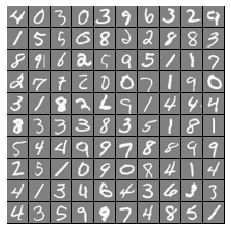
For this exercise, you will use logistic regression and neural networks to recognize handwritten digits (from 0 to 9). Automated handwritten digit recognition is widely used today - from recognizing zip codes (postal codes) on mail envelopes to recognizing amounts written on bank checks. This exercise will show you how the methods you've learned can be used for this classication task.

In the rst part of the exercise, you will extend your previous implemention of logistic regression and apply it to one-vs-all classication.

代码实现如下：

# -*- coding: utf-8 -*-
"""
Created on Wed Nov 20 15:19:25 2019

@author: Lonely_hanhan
"""
import scipy.io as sio
import numpy as np
import matplotlib.pyplot as plt
import scipy.optimize as op

input_layer_size = 400
num_labels = 10

''' =========== Part 1: Loading and Visualizing Data ============='''

# Load Training Data
print('Loading and Visualizing Data ...\n')

data = sio.loadmat('D:\exercise\machine-learning-ex3\machine-learning-ex3\ex3\ex3data1.mat')
X = data['X']
y = data['y']
m = X.shape[0]

def displayData(X):
    
    #Compute rows, cols
    [m, n] = X.shape
    example_width = round(np.sqrt(n)).astype(int)
    example_height = (n / example_width).astype(int)
    #Compute number of items to display
    display_rows = np.floor(np.sqrt(m)).astype(int)
    display_cols = np.ceil(m / display_rows).astype(int)
    
    #Between images padding
    pad = 1
    
    #Setup blank display
    display_array = - np.ones((display_rows * (example_height + pad), \
                            display_cols * (example_width + pad)))
    
    # Copy each example into a patch on the display array
    curr_ex = 0
    for j in range(display_rows):
        for i in range(display_cols):
            if curr_ex > m-1:
                break
            #Copy the patch
            #Get the max value of the patch
            max_val = np.max(np.abs(X[curr_ex]))
            display_array[j * (example_height + pad) + np.arange(example_height),\
                          i * (example_width + pad) + np.arange(example_width)[:, np.newaxis]] = \
                          X[curr_ex].reshape((example_height, example_width)) / max_val
            curr_ex += 1
        if curr_ex > m-1:
            break
    plt.figure()
    plt.imshow(display_array, cmap='gray', extent=[-1, 1, -1, 1])
    plt.axis('off')
    return
    
    


rand_indices = np.random.permutation(range(m)) #获取0-4999 5000个无序随机索引
selected = X[rand_indices[0:100], :]  #获取前100个随机索引对应的整条数据的输入特征
 
displayData(selected)   #调用可视化函数 进行可视化
 
input('Program paused. Press ENTER to continue')
    

''' =========== Part 2a: Vectorize Logistic Regression ============='''    
print('\nTesting lrCostFunction() with regularization')

def sigmond(z):
    return 1/(1+np.exp(-z))

def Irgradient(theta, X, y, lambdaE):
    m = len(y)
    theta1 = theta.T.copy()           # 因为正则化j=1从1开始，不包含0，所以复制一份，前theta(0)值为0 
    theta1[0] = 0
    grad = np.zeros((1, X.shape[1]))
    grad[0,0] = np.dot((sigmond(np.dot(theta, X.T))-y.T), X[:,0]) / m
    
    temp = np.array(theta1[1:]).reshape((1,theta1[1:].shape[0])) 
    grad[0 , 1:] = (np.dot((sigmond(np.dot(theta, X.T))-y.T), X[:,1:]) + np.dot(lambdaE, temp)) / m
    return grad

def lrCostFunction(theta, X, y, lambdaE):
    m = len(y) # number of training examples
    #You need to return the following variables correctly 
    ''' Cost '''
    J = 0
    
    theta1 = theta.T.copy()           # 因为正则化j=1从1开始，不包含0，所以复制一份，前theta(0)值为0 
    theta1[0] = 0
    J = ((-np.dot(np.log(sigmond(np.dot(theta, X.T))), y)) - np.dot(np.log(1 - sigmond(np.dot(theta, X.T))), (1-y))) / m \
    + lambdaE * np.dot(theta1.T, theta1)/ (2 * m)
    return J

''' Gradient '''
   

#Test case for lrCostFunction
theta_t = np.array([[-2, -1, 1, 2]])  
x_0 = np.ones((5, 1))
X_t = np.arange(1, 16).reshape((3, 5)).T / 10
X_t = np.hstack((x_0 , X_t)) # Add a column of ones to X
y_t = np.array([[1, 0, 1, 0, 1]])
y_t = y_t.reshape((5,1))
lambda_t = 3.0
grad = Irgradient(theta_t, X_t, y_t, lambda_t)
J = lrCostFunction(theta_t, X_t, y_t, lambda_t)
   

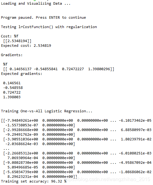
print('\nCost: %f\n', J)
print('Expected cost: 2.534819\n')
print('Gradients:\n')
print(' %f \n', grad)
print('Expected gradients:\n')
print(' 0.146561\n -0.548558\n 0.724722\n 1.398003\n')

''' =========== Part 2b: One-vs-All Training ============='''
print('\nTraining One-vs-All Logistic Regression...\n')

def oneVsAll(X, y, num_labels, lambda_train):
    m = X.shape[0]
    n = X.shape[1]
    #You need to return the following variables correctly 
    all_theta = np.zeros((num_labels, n + 1))
    #Add ones to the X data matrix
    X = np.c_[np.ones(m), X]
    J_ir = np.zeros((1, num_labels))
    
    for i in range(num_labels):
       #说明当i为0时，类别为10
        if i == 0:
            classn = 10
        else:
            classn = i
        
        y_train = np.array([1 if j == classn else 0 for j in y])
        resultreg = op.minimize(fun=lrCostFunction, x0=all_theta[i,:], args=(X, y_train, lambda_train), method='TNC',\
                        jac=Irgradient, options= {'maxiter': 100})
        J_ir[0,i]  = resultreg.fun
        all_theta[i,:] = resultreg.x
    return all_theta

lambda_train = 0.1
all_theta = oneVsAll(X, y, num_labels, lambda_train)    
        
print(all_theta)

''' =========== Part 3: Predict for One-Vs-All ============='''
def predictOneVsAll(all_theta, X):
    m = X.shape[0]
    num_labels = all_theta.shape[0]
    p = np.zeros(m)
    #You need to return the following variables correctly 
    #Add ones to the X data matrix
    X = np.c_[np.ones(m), X]
    
    y_p = sigmond(np.dot(X, all_theta.T))
    p = np.argmax(y_p, axis=1)
    p[p==0] = num_labels
    return p

pred = predictOneVsAll(all_theta, X)
#print(pred)
print('Training set accuracy:',sum(pred[:, np.newaxis] == y)[0] /5000 * 100,"%")

运行结果如下：

 

 

 在实现代码的过程中，发现了一些比以前更为简便的函数：

（1）round，floor，ceil

round()函数返回浮点数x的四舍五入值；

floor()函数返回数字的下舍整数，例如 np.floor(-45.17) = -46.0，np.floor(45.17) = 45.0；

ceil()函数返回数字的上入整数，例如np.ceil(-45.17) = -45.0，np.ceil(45.17) = 46.0；

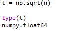
（2）astype()

用于array中数值类型转换，但是对于numpy.类型的函数，astype也是可以将其进行转换，例如：

（3）np.r_，np.c_，对于将X的列加一行以前的写法是利用np.hstack()

np.r_是按行连接两个矩阵，就是把两矩阵上下相加，要求列数相等

np.c_是按列连接两个矩阵，就是把两矩阵左右相加，要求行数相等

对于这段代码中的第三部分：Predict for One-Vs-All中类别的预测概率（这部分需要跟练习ex3_2进行对比）的自己的理解：

由于上述计算得到最优all_theta，数字的类别是根据0代表的是10,1代表的是1等，所以最后得到的概率也是根据这个规律进行的，即p[p==0] = 10 #第0类代表的就是数字10，这个跟练习ex3中第二部分中的类别的预测概率是不同的。

这里要感谢作者： NotFound1911 链接：https://blog.csdn.net/qq_24739717/article/details/88712085

为了记录自己的学习进度同时也加深自己对知识的认知，刚刚开始写博客，如有错误或者不妥之处，请大家给予指正。