


晚上鸟沒事,白天没鸟事
This is a sequel to my previous post about image classification using the NABirds data set provided by the Cornell Lab of Ornithology. In this article, I move beyond simple classification, and consider object detection, which might be better termed image or object localization. Not only am I trying to determine if a certain object is in a given picture, the detection component, but I am also trying to figure out where, i.e. the location, in the image the object happens to be.
这是我以前关于使用康奈尔鸟类学实验室提供的NABirds数据集进行图像分类的文章的续篇。 在本文中,我超越了简单的分类,而是考虑了对象检测 ,它可能更好地称为图像或对象定位。 我不仅试图确定给定图片中是否存在特定对象(检测组件),而且还试图找出该对象恰好在图像中的位置,即位置。
My own opinions notwithstanding, object detection is the term used universally in the literature and I will adhere to convention.
尽管有我自己的观点,但对象检测是文献中普遍使用的术语,我将遵循惯例。
A detailed discussion of the NABirds data can be found in the earlier article; I will merely review the highlights here. There are 48,562 images, more or less evenly split between training and validation sets, of 404 species of birds. Apart from the images, there is a significant amount of metadata, including several levels of taxonomy and annotations for male/female, juvenile/adult, and other color morphs where appropriate. The end result is 555 categories at the finest level. At the coarsest level, which will be of more interest here, there are 22 categories. At no level is the data even close to being balanced; some categories are very common and others are exceedingly rare.
有关NABirds数据的详细讨论,请参见前面的文章。 我将仅在这里回顾重点内容。 有404种鸟类的48,562张图像,或多或少均匀地分布在训练集和验证集之间。 除图像外,还有大量的元数据,包括几种分类法和相应的男/女,少年/成人和其他颜色变形的注释。 最终结果是555个类别的最佳分类。 在最粗糙的层次上,这里有22个类别。 数据甚至没有达到平衡的水平。 有些类别非常常见,而另一些则极为罕见。
The goal of this project is twofold. First, I simply want to predict a bounding box containing a bird in the image. There is only one detection class, bird, and the model has to find where the avian is in the picture. The second task is to locate the bird, and predict which of the 22 top level categories, which roughly correspond to Orders in taxonomy, the bird belongs to. The categories, listed alphabetically by common name description, with image counts are listed below. Note that perching birds, which account for more than half of all bird species, is, by far, the largest group. Astute naturalists will also notice that one order, Charadriiformes (i.e. shorebirds), has been divided into several categories.
该项目的目标是双重的。 首先,我只想预测图像中包含鸟的边界框。 只有一个检测类,鸟类,模型必须找到图中的禽类位置。 第二项任务是定位鸟类,并预测该鸟类所属的22个顶级分类中的哪一个(大致与分类法中的顺序相对应)。 下面列出了按通用名称描述按字母顺序列出的类别以及图像计数。 请注意,到目前为止, 栖息的鸟类最多,占所有鸟类总数的一半以上。 精明的博物学家还将注意到,一个象甲纲目(即shore鸟)已被分为几类。
边界框 (Bounding Boxes)
Each image has only one labeled bird and one bounding box containing it. A bounding box is a small rectangle containing the object in the image the model is searching for and as little else as possible. There are three ways to label bounding boxes, all involving four coordinates. The simplest is to use the coordinates of the upper left and lower right corners of the box. (By convention, the upper left corner of the image is (0, 0) and the upper right is (width, height)). Alternatively, the lower right corner can be replaced by the height and width of the box. A third, and more numerically stable, system is to use the height and width, but replace the upper left corner with the center of the box. All three methods are used by object detection networks as inputs, but most convert to the third system when training the neural net.
每个图像只有一个标记的鸟和一个包含它的边界框。 边界框是一个小矩形,其中包含模型正在搜索的图像中的对象,并且其他内容越少越好。 有三种标记边界框的方法,所有方法都涉及四个坐标。 最简单的方法是使用框的左上角和右下角的坐标。 (按照惯例,图像的左上角为(0,0),右上角为(宽度,高度))。 或者,可以用盒子的高度和宽度代替右下角。 第三个也是数值上更稳定的系统是使用高度和宽度,但将左上角替换为框的中心。 物体检测网络将这三种方法都用作输入,但是在训练神经网络时,大多数方法会转换为第三种方法。

The above picture is a good example. The bounding box completely encloses the sharp-shined hawk except for part of its tail (tails are tricky when bounding animals). The box is almost as tight as possible while still enclosing the whole animal. In our three notation schemes the box would be encoded as follows:
上图是一个很好的例子。 包围盒完全包围了锐利的鹰,除了它的部分尾巴(包围动物时,尾巴很棘手)。 盒子几乎是尽可能紧的,同时仍然封闭了整个动物。 在我们的三种注释方案中,框的编码如下:
- upper left, lower right = (141, 115), (519, 646). 左上,右下=(141,115),(519,646)。
- upper left, width, height = (141, 115), 378, 531. 左上,宽度,高度=(141,115),378,531。
- center, width, height = (330, 380.5), 378, 531. 中心,宽度,高度=(330,380.5),378,531。
In practice, the coordinates are usually scaled to be a percentage of the width and the height (i.e. between 0 and 1). It is also common to use log scale transform of the height and the width of the boxes, as small errors in predicting the size of large boxes are less serious than small errors predicting the size of small boxes.
实际上,通常将坐标缩放为宽度和高度的百分比(即0到1之间)。 由于箱子的高度和宽度的对数刻度变换也很常见,因为预测大箱子的尺寸时的小误差不如预测小箱子的尺寸时的小误差严重。
In principle, an image can contain any number of bounding boxes enclosing any number of different categories of object. I’m fortunate that each image in NABirds has only one box. It has little effect on the training, but will make evaluation of the model somewhat simpler.
原则上,图像可以包含任意数量的包围盒,其中包含任意数量的不同类别的对象。 我很幸运,NABirds中的每个图像只有一个框。 它对训练的影响很小,但是会使模型的评估更简单。
物体检测网络 (Object Detection Networks)
Neural networks for object detection build on the basic architecture of neural networks for image classification. Image classification networks consist of an amazingly complex combination of convolutional layers, skip connections, inception layers (a sort of fractal layers-within-layers architecture), pooling layers, batch normalization, dropout, and squeeze-and-excitation components, but the final layers are simple. A global average pooling (GAP) layer collapses the final tensor to a single feature vector, optional batch normalization and dropout layers provide regularization, and a final dense layer, usually with softmax activation, provides the final classification. Arguably, a neural network for image classification is simply a complicated feature extractor followed by logistic regression, with the GAP layer marking the transition point. Most object detection networks work by removing the top of the networks, starting with the GAP layers, and replacing it with something a bit more complicated.
用于对象检测的神经网络建立在用于图像分类的神经网络的基本架构之上。 图像分类网络由卷积层,跳过连接,初始层(某种分形层-层内体系结构),池化层,批处理归一化,辍学以及挤压和激发组件的惊人复杂组合组成,但最终图层很简单。 全局平均池(GAP)层将最终张量折叠为单个特征向量,可选的批处理归一化和辍学层提供了正则化功能,而最终的密集层(通常具有softmax激活)提供了最终分类。 可以说,用于图像分类的神经网络只是一个复杂的特征提取器,然后进行逻辑回归,GAP层标记了过渡点。 大多数对象检测网络的工作方式是:从GAP层开始,移除网络的顶部,然后将其替换为更复杂的东西。
That something involves anchor boxes. Each of these boxes is centered at some point in the image and has height and width some fraction of the image. Normally, there is a grid of anchor boxes of a given size that covers the entire image. A full set of anchor boxes is a collection of grids of varying resolutions; the larger the boxes, the fewer the grid points. An anchor box is a positive anchor for a given class if its overlap with an input bounding box for that class is large enough. If the overlap is too small the anchor is a negative anchor, and anything between these bounds is ignored. The typical measure for this overlap is IoU (Intersection over Union, which is exactly what it sounds like: the area of the overlap of the two boxes divided by their conbined area). Typical bounds are IoU > 0.7 for positive and IoU < 0.3 for negative.
那东西涉及锚盒。 这些框中的每个框都位于图像中某个点的中心,并且高度和宽度为图像的一部分。 通常,给定大小的锚点框网格覆盖整个图像。 全套锚框是各种分辨率的网格的集合。 框越大,网格点越少。 如果锚点框与给定类的输入边界框重叠,则该锚点框是该类的正锚点。 如果重叠太小,则锚点是负锚点,并且这些边界之间的所有内容都将被忽略。 这种重叠的典型度量是IoU(联合上方的交点,这听起来像是这样:两个盒子的重叠面积除以它们的合并面积)。 典型范围是正数的IoU> 0.7,负数的IoU <0.3。
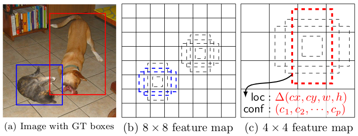
Before GAP is performed, the final output tensor could be seen as a grid of feature vectors, each one predicting the presence of an object in a small portion of the image. A very simple (a little too simple) object detection model could then just attach a classification layer to each vector in the grid as well as a second layer that outputs four box coordinates. The model could then be trained with a loss function that is the sum of the softmax classifier and an MSE regression loss on the box coordinates (usually the center, width, and height for numerical stability).
在执行GAP之前,最终的输出张量可以看作是特征向量的网格,每个预测特征在图像的一小部分中存在对象。 然后,一个非常简单(有点太简单)的对象检测模型可以将分类层附加到网格中的每个矢量,以及第二层输出四个框坐标。 然后可以使用损失函数来训练模型,该损失函数是softmax分类器和框坐标上的MSE回归损失(通常为数值稳定性的中心,宽度和高度)之和。
As I said, that’s a little too simple, but not by much. The model described above would correspond to the coarsest level of anchor boxes since the final tensor before GAP has a much smaller width and height than the original image. In the case of the old VGG16 network, a 224x224 image leaves a 7x7x512 box before final processing. I’d only be able to detect 49 possible bound boxes, one each for the 32x32 sub-images made by partitioning the original into a 7x7 grid. In practice, I need to be able to search for thousands of possible box centers, at several resolutions.
就像我说的那样,这有点太简单了,但并不是很多。 由于GAP之前的最终张量的宽度和高度比原始图像小得多,因此上述模型将对应于锚框的最粗糙级别。 对于旧的VGG16网络,在最终处理之前,一个224x224的图像会留在7x7x512的盒子中。 我只能检测49个可能的装订框,每个装订框对应于通过将原件分成7x7网格而制成的32x32子图像。 实际上,我需要能够以多种分辨率搜索成千上万个可能的盒子中心。
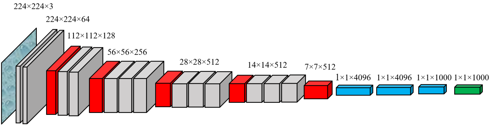
I can introduce finer resolutions by using some the network’s earlier layers. In this case I have 14x14, and 28x28 grids available to me. Since they’re earlier in the network, the features contain less information, but I can get around that by upsampling the later features and adding the results back in. Each layer would then correspond to a grid of anchor boxes. This is still a little too simple for modern object detection models, which learn complicated relationships between the various resolution layers. In the finest tradition of neural networks, the layers that combine the resolution layers can themselves be stacked together to form richer features.
我可以通过使用网络的某些较早的层来介绍更好的分辨率。 在这种情况下,我可以使用14x14和28x28的网格。 由于它们位于网络中较早的位置,因此这些功能包含的信息较少,但是我可以通过对更高版本的功能进行上采样并重新添加结果来解决此问题。然后,每个图层将对应于一个锚定框网格。 对于现代对象检测模型来说,这仍然有点太简单了,该模型学习了各种分辨率层之间的复杂关系。 在神经网络的最优良传统中,结合分辨率层的层本身可以堆叠在一起以形成更丰富的特征。

There are three more significant, although much simpler, changes that must be made before I have a good object detection network. First, softmax must be replaced by sigmoid at all classification points. Softmax does not really handle the absence of any object, which will be the most common output at most anchor points, so the presence or absence of each class must be predicted independently. Second, the classification and regression losses are on different scales; a weighting factor must be added in so that both responses train well. Depending on the model, class_loss + 10 * box_loss or class_loss + 50 * box_loss will work well. The third, and possibly simplest, addition is to have each anchor box center correspond to multiple anchor boxes of different aspect ratios.
在拥有良好的对象检测网络之前,还必须进行三个更重要的更改,尽管要简单得多。 首先,在所有分类点上,softmax必须替换为S型。 Softmax不能真正处理缺少任何对象的情况,这将是大多数锚点上最常见的输出,因此必须单独预测每个类的存在或不存在。 其次,分类损失和回归损失的规模不同。 必须添加一个加权因子,以便两个响应都能很好地训练。 根据型号,class_loss + 10 * box_loss或class_loss + 50 * box_loss会很好地工作。 第三种(可能是最简单的)添加方法是使每个锚框中心对应于不同长宽比的多个锚框。
高效饮食 (EfficientDet)
The basic premise of the EfficientNet series of networks is that a simple relationship between three major network parameters (number of layers, image resolution, and filters per layer) could be used to easily generate a family of models of various sizes for image classification, ranging from small models suitable for smartphones to the larger models necessary for state of the art accuracy. EfficientDet extends the same principle to object detection models. The basic EfficientNet backbones are used as feature extractors in the manner described above. Instead of a GAP layer at the end, the different resolution levels are further processed by a series of bidirectional feature pyramid networks (BiFPN). The number of BiFPN layers, and the number of channels per layer, scales up with the size of the backbone network. At the end are a few more convolution layers followed by classification and box prediction.
EfficientNet系列网络的基本前提是,可以使用三个主要网络参数(层数,图像分辨率和每层滤镜)之间的简单关系轻松生成用于图像分类的各种尺寸的模型系列从适用于智能手机的小型机型到满足最新技术精度的大型机型。 EfficientDet将相同原理扩展到对象检测模型。 基本的EfficientNet主干网以上述方式用作特征提取器。 代替最后的GAP层,通过一系列双向特征金字塔网络(BiFPN)进一步处理不同的分辨率级别。 BiFPN层的数量以及每层的通道数随骨干网的规模而扩大。 最后是更多的卷积层,然后进行分类和框预测。
Since I used EfficientNet for my previous project, EfficientDet seemed a natural choice for this project. This came with a few challenges. When I started working, the only viable option for running EfficientDet with Colab was based on PyTorch. (Tensorflow has since released their own implementation). Up until now, all my work had been done in Tensorflow. Learning to work in a new environment is always a challenge, but I didn’t mind that. The real downside to working in PyTorch was that I couldn’t use a TPU on Colab. Having recourse only to the GPU, I was forced to scale down the number of different models I could compare. To date, I have only run D0 through D2, each with the default input size. Object detection usually uses larger images than simple classification, which means batch sizes must be smaller, and thus learning rates must be smaller. I could only use batch sizes of 4 for the models. Initial learning rate was set at 0.0002 and dropped by half after each epoch where the validation loss didn’t improve. I gave the model the option of training up to 100 epochs, but usually found I could stop by epoch 50.
由于我在之前的项目中使用了EfficientNet,因此EfficientDet似乎是该项目的自然选择。 这带来了一些挑战。 当我开始工作时,与Colab一起运行EfficientDet的唯一可行选择是基于PyTorch。 (此后,Tensorflow已发布了自己的实现)。 到目前为止,我所有的工作都在Tensorflow中完成。 学习在新环境中工作始终是一个挑战,但我并不介意。 在PyTorch中工作的真正弊端是我无法在Colab上使用TPU。 仅依靠GPU,我不得不缩小我可以比较的不同模型的数量。 到目前为止,我只运行D0到D2,每个都使用默认输入大小。 与简单分类相比,对象检测通常使用更大的图像,这意味着批量必须较小,因此学习率必须较小。 我只能为模型使用4的批量大小。 初始学习率设置为0.0002,并且在每次验证有效性没有改善的时期之后降低一半。 我给模型提供了最多训练100个纪元的选项,但通常发现我可以在第50个纪元之前停下来。
前处理 (Preprocessing)
As with all image processing neural networks, object detection is very dependent on good image preprocessing. Most of the important preprocessing operations involve transformations, such as shifts and zooms, that affect the bounding box just as much as the image. Fortunately, there’s a package, albumentations, that can handle this. I’ve no idea what, if anything, albumentations are supposed to be (and it looks like the spell checker is just as stumped) but the package consists of functions that ensure any transformation applied to an image is also applied to the associated bounding box and/or image mask in the case of image segmentation problems.
与所有图像处理神经网络一样,对象检测非常依赖于良好的图像预处理。 大多数重要的预处理操作都涉及到诸如边框和缩放之类的变换,这些变换对边界框的影响与图像一样重要。 幸运的是,有一个软件包albumentations可以处理此问题。 我不知道应该是什么(如果有的话)唱片集(看起来像拼写检查器一样残缺),但是该包包含确保将应用于图像的任何转换也应用于关联的边框的功能和/或在出现图像分割问题时使用图像遮罩。
NABirds images come in a variety of sizes, with an upper bound on height and width of 1024. About half have one side of length 1024 and the other somewhere between 600 and 900. Batch processing requires a fixed input size. This is easy enough for training data, since I take a random square crop out of the image anyway, but is a bit trickier for validation. Since I don’t want to lose any information by cropping the validation images, I instead rescale so that the longer dimension matches the input size and then pad the smaller dimension until the image in is a square.
NABirds图像具有多种尺寸,高度和宽度的上限为1024。大约一半的一侧长度为1024,另一侧的长度在600到900之间。批处理需要固定的输入尺寸。 这对于训练数据来说很容易,因为无论如何我都会从图像中截取随机的方形作物,但是对于验证来说有点棘手。 由于我不想通过裁剪验证图像而丢失任何信息,因此我重新缩放比例,以使较长的尺寸与输入尺寸匹配,然后填充较小的尺寸,直到图像变为正方形为止。

The set of transforms I use on the training data is listed below.
下面列出了我在训练数据上使用的一组变换。
The first operation takes a random rectangular crop from the original image ranging in size between the full image and 10%, with an aspect ratio between 4:3 and 3:4, and reshapes it to a square of the appropriate size. I always use the default input size of whichever EfficientDet network I’m using.
第一个操作是从原始图像中获取一个随机的矩形裁剪,其尺寸在整个图像和10%之间,长宽比在4:3和3:4之间,并将其整形为适当大小的正方形。 我始终使用我正在使用的任何EfficientDet网络的默认输入大小。
Stage two changes the hue or brightness, but not both, with 90% probability (i.e. one time out of ten it does nothing). Stage three changes the image to greyscale 1% of the time. The next three operations are flips along the vertical, horizontal, and diagonal axes, each with 50% probability. Cutout will replace some small square in the image with zeros; it functions like dropout on later layers. A sample of training images produced by these transformations is below.
第二阶段以90%的概率改变色调或亮度,但不能同时改变两者(即十分之一改变了它什么也不做)。 第三阶段会在1%的时间内将图像更改为灰度。 接下来的三个操作是沿垂直,水平和对角线轴的翻转,每个翻转的概率为50%。 抠图会将图片中的一些小方块替换为零; 它的功能就像在以后的层上退出。 这些转换产生的训练图像样本如下。
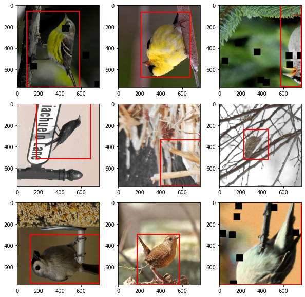
Eagle-eyed readers will notice that all of these images contain bounding boxes, although in one case the box is now the full image. What happens if the random crop does not contain the box at all? Very simply, I try again. The preprocessing code makes as many as 100 attempts to produce a crop with a bounding box before falling back on a simpler default, which merely performs the resize operation on the whole image.
老鹰眼的读者会注意到,所有这些图像都包含边界框,尽管在某些情况下,该框现在是完整图像。 如果随机作物根本不包含盒子,会发生什么? 很简单,我再试一次。 预处理代码最多会尝试100次使用边界框生成作物,然后再使用更简单的默认值,该默认值仅对整个图像执行调整大小操作。
My validation transforms are below.
我的验证转换如下。
All this does is pad the image with zeros until I get a square, and then resizes to fit the model. The end result of its handiwork is below.
所有这些操作是用零填充图像,直到得到一个正方形,然后调整大小以适合模型。 手工的最终结果如下。

训练 (Training)
PyTorch does not have the Keras frontend available to Tensorflow, which means training a model requires a bit more manual work. The key idea is still fairly simple. For each batch of training data forward propagate to get current predictions and then back propagate to update the parameters. The full Fitter class I used has too much boilerplate code for this article, but I can share the loop that trains one epoch.
PyTorch没有Tensorflow可用的Keras前端,这意味着训练模型需要更多的手动工作。 关键思想仍然很简单。 对于每批训练数据,向前传播以获取当前预测,然后向后传播以更新参数。 我在本文中使用的完整Fitter类具有太多样板代码,但是我可以共享训练一个纪元的循环。
After each training epoch, a similar loop performs validation. If the new parameters are an improvement, the model is saved.
在每个训练时期之后,类似的循环执行验证。 如果新参数有所改进,则将保存模型。
验证方式 (Validation)
Object detection validation is not a simple matter. Unlike image classification, which produces one probability for each category, object detection produces a separate probability and bounding box for each category and anchor box in the output. That’s a lot of numbers. Most of which can can be easily discarded simply by thresholding, i.e. if the score for a certain category in a certain anchor is low enough, we can ditch it without a second thought. In practice, that will be the case for all categories in most of the anchor boxes and most categories in all of the anchor boxes. That still leaves the possibility of multiple bounding boxes marked as positive IDs. If the positive categories don’t match the real categories then there is an obvious misclassification, but if the categories match, it’s necessary to consider the accuracy of the bounding box as well.
对象检测验证不是一件容易的事。 与图像分类不同,图像分类为每个类别生成一个概率,而对象检测为输出中的每个类别和锚定框生成一个单独的概率和边界框。 有很多数字。 仅通过阈值就可以轻松丢弃其中的大多数内容,即,如果某个锚中某个类别的得分足够低,我们可以不加考虑就放弃它。 实际上,大多数锚定框中的所有类别和所有锚定框中的大多数类别都是这种情况。 仍然有可能将多个边界框标记为正ID。 如果肯定类别与真实类别不匹配,则存在明显的误分类,但如果类别匹配,则也必须考虑边界框的准确性。
As described above, object detection models rely on anchor boxes. After the model is trained, each one of these anchors has an output. Most can be ignored simply because of their low confidence score. It’s also possible that two (or more) neighboring anchors will produce positive output for the same class. In this case, the bounding boxes will be very similar and only one needs to be saved, the one with the highest confidence score. Non-max suppression is the standard algorithm for removing redundant bounding boxes.
如上所述,对象检测模型依赖于锚框。 训练模型后,这些锚点中的每一个都有一个输出。 大多数人仅凭其低置信度就可以忽略。 两个(或更多)相邻的锚也可能为同一类产生正输出。 在这种情况下,边界框将非常相似,并且仅需保存一个边界框,即具有最高置信度得分的边界框。 非最大抑制是删除冗余边界框的标准算法。
Only now can I get down to the business of comparing the model’s output to the ground truth. I have something of an advantage here knowing that I have only one bounding box per image; I can evaluate by only considering the predicted bounding box with the highest confidence. The metrics used for measuring accuracy deal specifically with precision and recall so I’ll have to define true positive, false positive, and false negative for object detection.
直到现在,我才可以从事将模型的输出与基本事实进行比较的工作。 我知道每个图像只有一个边界框,这对我有好处。 我只能通过考虑具有最高置信度的预测边界框来进行评估。 用于测量准确性的度量标准专门涉及精度和召回率,因此我必须为对象检测定义真阳性,假阳性和假阴性。
- True Positive — Predicted category matches ground truth and IoU is greater than some threshold. 真实肯定-预测类别与实际情况相符,并且IoU大于某个阈值。
- False Positive — Predicted category matches ground truth but the IoU is below the threshold. 误报-预测类别与实际情况相符,但IoU低于阈值。
- False Negative — Predicted category does not match ground truth or no category is predicted. 假阴性-预测类别与基本事实不匹配,或者没有预测类别。
Precision is the ratio of the true positives to all predicted positives and recall is the ratio of true positives to the ground truth results. In layman’s terms, precision is the percentage of true predictions that are accurate and recall is the percentage of positive classes identified.
精确度是真实阳性与所有预测阳性的比率,召回率是真实阳性与真实结果的比率。 用外行的话来说,精度是指准确的真实预测所占的百分比,召回率是所标识的肯定类别的百分比。
Object detection models are evaluated by calculating precision at various IoU thresholds (0.5 and 0.75 are popular) and by averaging the precision (the seemingly redundantly named mean average precision) over a range of IoU thresholds (usually 0.5 to 0.95 in increments of 0.05.) Similar metrics can be calculated for recall.
通过在各种IoU阈值(通常为0.5和0.75)下计算精度并在一系列IoU阈值(通常为0.5至0.95,以0.05为增量)上平均精度(看似多余的平均平均精度)来评估对象检测模型。可以计算类似的指标以进行召回。
Single Class Detection
单类检测
The simpler of my two problems is simply to find where in the image there is a bird and returns the box containing it. I tried three different models, D0 through D2 in the EfficientDet family, using the bounding box with the highest confidence score as the prediction. I only allow confidence scores above 0.5; a few images sufficiently confuse the models that no bounding box meets that threshold, so there are a few false negatives.
我的两个问题中,最简单的一个就是简单地找到图像中的鸟儿,然后返回包含它的盒子。 我尝试了三种不同的模型,即EfficientDet系列中的D0到D2,使用具有最高置信度得分的边界框作为预测。 我只允许置信度得分高于0.5; 一些图像足以使模型混淆,以至于没有边界框满足该阈值,因此存在一些假阴性。
False positives are more interesting. As a metric, IoU has to wear a couple different hats. It says that the predicted box must cover a certain amount of the ground truth box, but also that the ground truth box must cover a certain amount of the predicted box. A low IoU may mean that the model detected a bird in the wrong part of the image, but may also mean that the model found the bird but wasn’t precise enough (i.e. the box was too big.) More often than not, a false positive will be a case where the bird was detected, and will be in the bounding box, but the predicted coordinates were not good enough.
误报更有趣。 作为衡量标准,IoU必须戴上几顶不同的帽子。 它说预测框必须覆盖一定量的地面实测框,而且地面实测框必须覆盖一定量的实测框。 IoU较低可能意味着模型在图像的错误部分检测到了一只鸟,但也可能意味着该模型找到了那只鸟,但不够精确(即盒子太大)。误报将是在检测到鸟类的情况下,并将其放在边界框中,但预测的坐标不够好。
Intuitively, an IoU score of 0.5 might seem a little low. It’s worth looking at some examples to see what different IoU thresholds look like. Remember, images are in two dimensions. Our minds have trouble recognizing when area or volume doubles when more than one dimension is changing at a time. Let’s look at what IoU=0.8 amounts to in real life.
凭直觉,IoU得分为0.5似乎有点低。 值得看一些示例,以了解不同的IoU阈值是什么样的。 请记住,图像是二维的。 当一次更改多个维度时,我们的思维难以识别面积或体积翻倍。 让我们看一下IoU = 0.8在现实生活中的含义。

Anyone looking at these images would probably guess that the overlap is better than 90%, but in reality its a little under 80% in all cases. This suggests that 0.8, which would be considered a mediocre value for a lot of metrics, is not that bad for bounding boxes. It’s also worth noting that the predicted box is often better than the “ground truth.” Human annotators have their limits.
任何查看这些图像的人都可能会猜想重叠率要好于90%,但实际上在所有情况下其重叠率都不到80%。 这表明0.8(对于许多度量标准而言,是中等值)对于边界框而言并不算太坏。 还要注意的是,预测的框通常比“基本事实”要好。 人类注释者有其局限性。
Even cases where the IoU is a measly 0.5 often look okay to these human eyes.
即使IoU仅为0.5,在这些人眼中通常看起来也还不错。

Both of these examples used predictions from EfficientDetD0. As I increase from D0 to D2, the accuracy improves modestly.
这两个示例都使用了来自EfficientDetD0的预测。 当我从D0增加到D2时,精度会适度提高。
Using an IoU of 0.5 as the threshold, the models have near perfect precision. Only in a few cases does the predicted bounding box not overlap the ground truth adequately. Even at the higher threshold of 0.75 prediction and ground truth match at least nine times out of ten. The mean average precision, which averages precision at IoU threshold between 0.5 and 0.95, is a bit lower since precision above IoU=0.9 drops precipetously.
使用0.5的IoU作为阈值,模型具有接近完美的精度。 仅在少数情况下,预测边界框才会与地面实况充分重叠。 即使在0.75的较高阈值下,预测和基本事实也至少匹配十分之九。 由于在IoU = 0.9以上的精度会急剧下降,因此平均平均精度(在IoU阈值处的平均精度在0.5和0.95之间)要低一些。
Mean average recall is also nearly perfect since only a couple hundred images do not have any bounding boxes with confidence score at least 0.5.
平均平均召回率也几乎是完美的,因为只有几百张图像没有置信度至少为0.5的边界框。
Looking just at the metrics, the models appear to be performing well. As the model size increases accuracy increases modestly but consistently. Looking at the output, I think the models might even be doing better than the numbers suggest. In a number of cases, the predicted bounding boxes are clearly better than the human labeled ground truth. In others, the predicted boxes are too large simply because the model assumes the bird extends behind a branch, a common enough situation. In one comical case, the predicted bounding box does not overlap the ground truth because it catches the bird’s reflection (in retrospect, allowing vertical flips in training may have been unwise). In another, the predicted box finds a second bird the annotator missed. I think that if the ground truth labels had been a little cleaner, the models’ performance would look even better.
仅查看指标,模型似乎表现良好。 随着模型尺寸的增加,精度会适度但持续增加。 从输出来看,我认为这些模型甚至可能比数字所暗示的要好。 在许多情况下,预测的边界框明显优于人类标记的地面实况。 在其他情况下,预测框太大是因为该模型假设鸟类在分支后面延伸,这是很常见的情况。 在一个可笑的情况下,预测的边界框不会与地面真相重叠,因为它捕获了鸟类的反射(回想起来,允许垂直翻转训练可能是不明智的)。 在另一个框中,预测框找到注释者错过的第二只鸟。 我认为,如果地面真相标签稍微干净一点,模型的性能就会更好。

Multi Class Detection
多类别检测
There are 22 top level category in Cornell’s data set, each corresponding to and order or family of birds and each with common names provided. Adding category detection complicates the classification (the what) component of an object detection model, but has less effect on the separate localization (the where) component. Since I’ve increased the number of positive classes from 1 to 22, I need to drop the threshold at which I consider a prediction score to be a positive match. I’m still dropping everything except the highest score (one bounding box per image) so I can take the relatively low score of 0.1 as a positive prediction.
康奈尔(Cornell)数据集中有22个顶级类别,每个类别分别对应鸟类,鸟类或鸟类,并提供共同的名称。 添加类别检测会使对象检测模型的分类(内容)复杂化,但对单独的本地化(位置)成分的影响较小。 由于我将肯定类别的数量从1增加到22,因此我需要降低将预测分数视为肯定匹配的阈值。 除了最高分数(每幅图像一个边界框)之外,我仍然会丢弃所有内容,因此我可以将0.1的较低分数作为肯定的预测。
How did I pick 0.1? Random guessing would give me just under 0.05; I doubled that, figuring that confidence scores twice random wouldn’t happen very often by chance. The results were favorable, so I stuck with it.
我如何选择0.1? 随机猜测会给我不到0.05; 我翻了一番,认为信心得分随机两次是不会偶然发生的。 结果不错,所以我坚持了下来。
It should come as no surprise that accuracy varies among the classes more or less in direct proportion to the number of images in the class. Since I made no attempt to equalize the data in training, the six classes with double digit image totals got two positive IDs in three models between them. Meanwhile, perching birds is at 97–98%. One gratifying result is that in the middle range, orders with between 300 and 1000 images, increasing the model size could have a dramatic impact. The true positive rate could jump 10–20% (more in the case of frigatebirds). Full true positive results are below.
毫无疑问,精度在类别之间或多或少地与类别图像的数量成正比地变化。 由于我在训练中没有尝试过均衡数据,因此具有两位数图像总数的六个类别在它们之间的三个模型中获得了两个正ID。 同时,鸟类的栖息率达到97-98%。 一个令人欣喜的结果是,在中间范围内,订购300至1000张图像,增加模型尺寸可能会产生巨大影响。 真正的阳性率可能会跳升10%至20%(对于护卫舰而言则更高)。 完全正确的正面结果如下。
The standard procedure in multi-class object detection problems is to compute average precision by averaging the precision over all classes. Given the level of class imbalance, I thought it would be instructive to compute an “unweighted” average precision over the whole data set. This will, of course, give me larger numbers than the standard weighted precision. I think both data points have some value.
多类对象检测问题中的标准过程是通过平均所有类的精度来计算平均精度。 考虑到类不平衡的程度,我认为在整个数据集上计算“未加权”平均精度将是有益的。 当然,这将给我比标准加权精度更大的数字。 我认为两个数据点都有一定价值。
Remember that a false positive is when the predicted order matches the ground truth, but the IoU of the predicted and ground truth boxes is too low.
请记住,假阳性是指预测的顺序与基本事实相匹配,但是预测和基本事实框的IoU太低。
Precision is lower than it is for the single class detectors, as expected, and increases slowly as the model increases, also as expected. The weighted (i.e. standard) average precision is much lower, but also increases at a faster rate than the unweighted metric. This reflects the fact that accuracy jumps dramatically for the mid-sized classes. The distribution of IoU values is pretty similar for both sets of models; almost all the decrease in accuracy is a reflection of the model now having to distinguish between 22 orders.
正如预期的那样,其精度低于单类探测器的精度,并且随着模型的增长(也与预期的一样)而缓慢增加。 加权(即标准)平均精度要低得多,但也比未加权度量提高了更快的速率。 这反映了一个事实,即中型班级的准确性急剧上升。 两组模型的IoU值分布都非常相似。 几乎所有精度的下降都反映出该模型现在必须区分22个阶次。
Further Work
进一步的工作
Any good experiment opens up the door to new questions. In this case, I can think of several. Assuming I can keep the batch size high enough (i.e. find a way to use TPUs) how would increasing the model size beyond D2 affect accuracy? I had made one experiment with D3, but was forced to cut the already small batch size in half. The end result was a lower recall and precision scores falling back to D0 levels. As I’d made no other changes, it seems the batch size was entirely responsible for that.
任何好的实验都会打开新问题的大门。 在这种情况下,我可以想到几个。 假设我可以保持足够大的批次大小(即找到一种使用TPU的方法),将模型大小增加到D2以上将如何影响准确性? 我用D3做过一个实验,但被迫将已经很小的批处理量减少一半。 最终结果是较低的召回率和精确度得分降至D0级。 由于我没有进行其他更改,因此似乎批量大小完全由该原因引起。
I’ve long suspected that larger models need lower learning rates. Would D3 and higher work better with a lower learning rate?
长期以来,我一直怀疑较大的模型需要较低的学习率。 D3和更高的水平会在学习率较低的情况下更好地工作吗?
What happens if, instead of 22 categories, I use all 404 species, or even all 555 classes? Everything I’ve seen about object detection suggests that it does not comfortably handle as many classes as image classification. Not yet, anyway.
如果我不使用22个类别,而是全部使用404种,甚至全部555个类别,会发生什么情况? 我所看到的有关对象检测的所有内容都表明,它不能舒适地处理像图像分类一样多的类。 仍然没有。
Perhaps the most useful test of the above algorithms would be to test them on some other set of bird data, such as the birds in the various iNaturalist data sets.
上述算法最有用的测试可能是在其他鸟类数据集(例如各种iNaturalist数据集中的鸟类)上对其进行测试。
晚上鸟沒事,白天没鸟事


 1449
1449


 被折叠的 条评论
为什么被折叠?
被折叠的 条评论
为什么被折叠?
 到【灌水乐园】发言


