


用于细粒度零样本学习的堆叠语义引导注意力模型
Stacked Semantics-Guided Attention Model for Fine-Grained Zero-Shot Learning
Stacked Semantics-Guided Attention Model for Fine-Grained Zero-Shot Learning
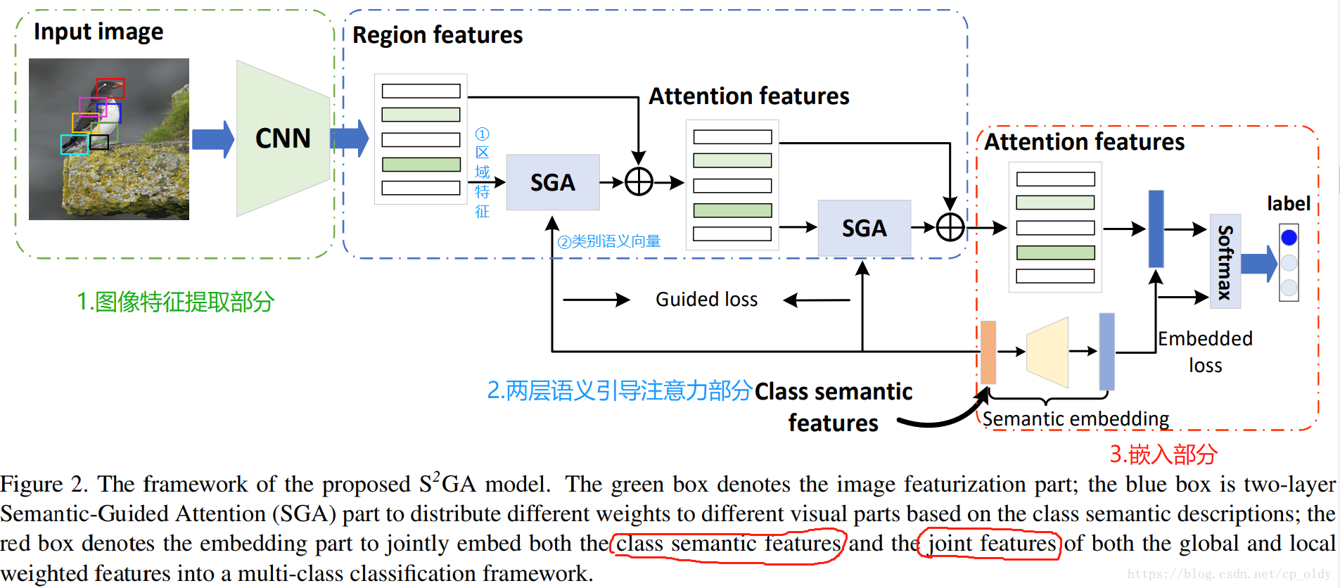
Abstract: Zero-Shot Learning (ZSL) is achieved via aligning the semantic relationships between the global image feature vector and the corresponding class semantic descriptions. However, using the global features to represent fine-grained images may lead to sub-optimal results since they neglect the discriminative differences of local regions. Besides, different regions contain distinct discriminative information. The important regions should contribute more to the prediction. To this end, we propose a novel stacked semantics-guided attention ( S 2 G A S^2GA S2GA) model to obtain semantic relevant features by using individual class semantic features to progressively guide the visual features to generate an attention map for weighting the importance of different local regions. Feeding both the integrated visual features and the class semantic features into a multi-class classification architecture, the proposed framework can be trained end-to-end. Extensive experimental results on CUB and NABird datasets show that the proposed approach has a consistent improvement on both fine-grained zero-shot classification and retrieval tasks.
零样本学习是通过对齐全局图像特征向量和对应的类别语义描述之间的语义关系实现的。然而,使用全局特征来表示细粒度图像可能会导致次优结果,因为这种表示忽略了局部区域的判别性差异。除此之外,不同区域包含了不同的判别性信息。重要的区域对预测结果贡献更大。为此,我们提出了一种新颖的堆叠语义引导注意力( S 2 G A S^2GA S2GA)模型,通过使用单独的类别语义特征来逐步引导视觉特征,生成一个用于衡量不同局部区域重要性的注意力图来获得语义相关特征。将集成的视觉特征和类别语义特征输入到多分类架构中,对提出的框架进行端到端的训练。在CUB和NABird数据集上的大量实验结果表明,所提出的方法在细粒度零样本分类和检索任务方面都有一致的提升。
亮点:使用加权局部特征来执行ZSL任务
结论1: 细粒度图像的视觉特征应该使用局部(细粒度)特征,而不是全局特征,来增加它的判别性
结论2:不同局部特征对最终的预测贡献不同。而对于不同的预测任务,不同局部区域的贡献应该也不同。也就是说,对于细粒度分类任务和细粒度ZSL任务来说,不同区域的贡献也是不同的。
结论3:因为ZSL任务是通过视觉语义的语义关系对齐实现的,所以不同区域的重要性是指它们对这个对齐的重要性。也就是说哪个区域对视觉语义映射重要,它就对ZSL任务重要。而区域特征是视觉特征,它对视觉语义映射重要,也就是要让这个特征经过映射能够更好地实现分类。论文的想法是,使得局部特征和语义相关,局部特征和语义相关性越大,那么它在最终的预测过程中,就能更准确的映射到类别语义描述上。
问题:1)attention map 是什么?PI
2)individual怎么翻译?单独的类
问题定义
细粒度零样本问题。

如图1所示,全局特征仅捕获一些整体信息,相反,区域特征捕获局部信息,并且局部特征与类别语义描述更相关。
Motivation:当试图识别未见类别图像时,人们更多关注基于关键类别语义描述的信息区域。此外,人类通过排除不相关的视觉区域并以渐进的方式定位最相关的视觉区域来实现语义对齐。
零样本问题中,模型是如何学习已知类和未知类的关系的?
答:通过语义关系,具体来讲就是定义的语义空间,比如属性空间、词向量空间或者描述空间。已知类和未知类共享语义空间,如果已知类的视觉语义映射比较好的话,模型在未知类的的泛化性能就好。
方法
多层注意力机制

创新点:通过语义引导加权不同区域。
语义如何嵌入网络?
f - 局部嵌入网络
输入:局部特征
V
I
V_I
VI
输出:隐空间的特征,
f
(
V
I
)
=
h
(
W
I
,
A
V
I
)
f(V_I)=h(W_{I, A} V_I)
f(VI)=h(WI,AVI)
g - 语义引导网络
输入:融合局部特征(全局)
V
G
V_G
VG + 类别语义向量
s
s
s
输出:
g
(
V
G
)
=
h
(
W
G
,
A
h
(
W
G
,
S
V
G
)
)
g(V_G)=h(W_{G, A}h(W_{G, S} V_G))
g(VG)=h(WG,Ah(WG,SVG))
Fusion是什么操作?
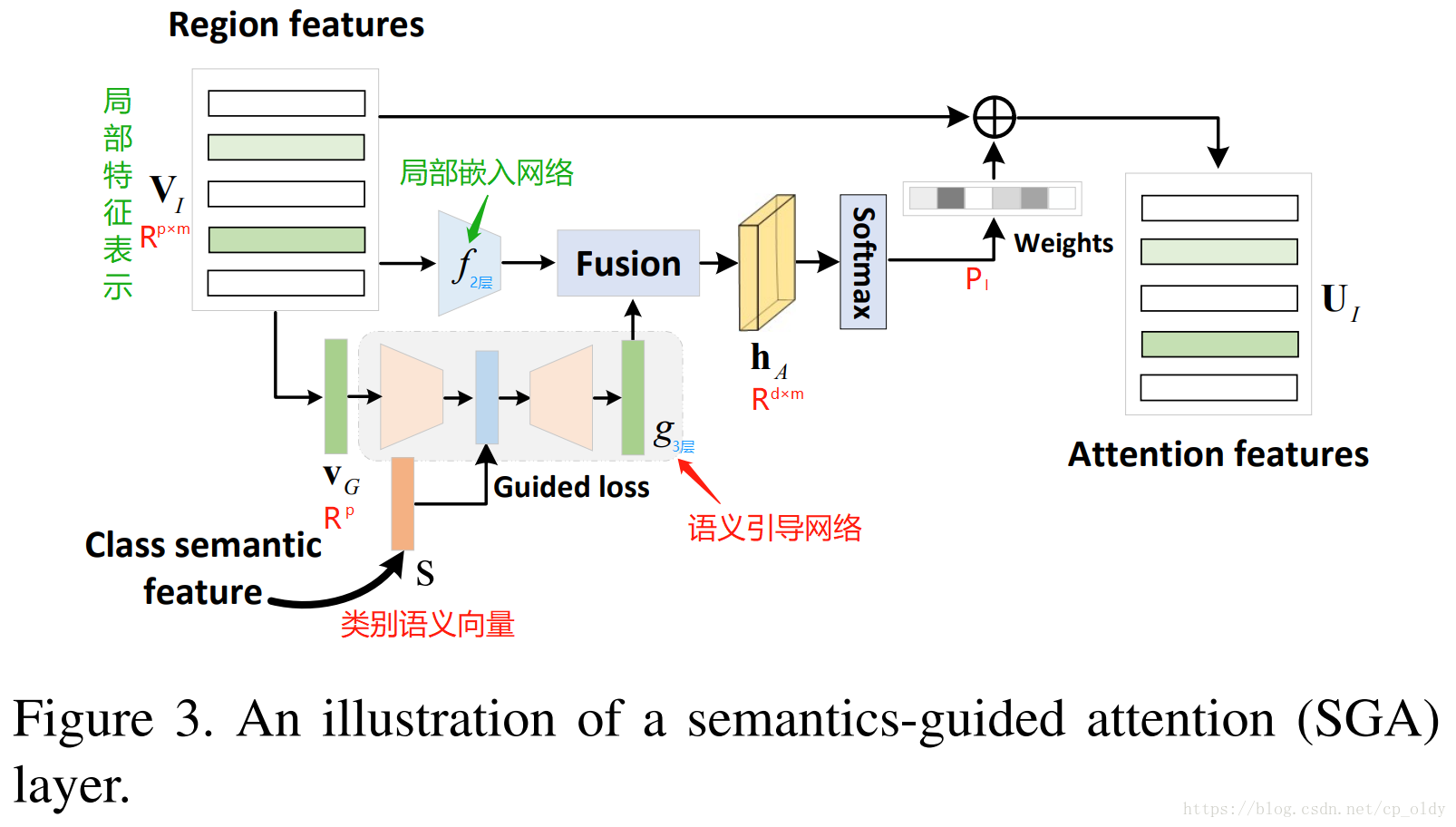
h A = t a n h ( f ( V I ) ⊕ g ( V G ) ) (1) h_A=tanh(f(V_I) \oplus g(V_G)) \tag {1} hA=tanh(f(VI)⊕g(VG))(1)
p I = s o f t m a x ( W P h A + b P ) (2) p_I=softmax(W_Ph_A+b_P) \tag {2} pI=softmax(WPhA+bP)(2)
h
A
∈
R
d
×
m
h_A \in R^{d \times m}
hA∈Rd×m是隐含空间的融合特征
V
I
∈
R
p
×
m
V_I \in R^{p \times m}
VI∈Rp×m 是区域特征,
m
m
m个
p
p
p维的区域特征向量
V
G
∈
R
p
V_G \in R^p
VG∈Rp 是全局特征
⊕
\oplus
⊕表示按像素乘法,论文里讲是
f
(
V
I
)
f(V_I)
f(VI)的每列和
g
(
V
G
)
g(V_G)
g(VG)每个元素相乘。
代码里是矩阵加
p I ∈ R m p_I \in R_m pI∈Rm是不同区域的权值(概率)
f ( V I ) = h ( W I , A V I ) (3) f(V_I)=h(W_{I, A} V_I) \tag {3} f(VI)=h(WI,AVI)(3)
g ( V G ) = h ( W G , A h ( W G , S V G ) ) (4) g(V_G)=h(W_{G, A}h(W_{G, S} V_G)) \tag {4} g(VG)=h(WG,Ah(WG,SVG))(4)
h h h是一个非线性函数(实验中使用ReLU), W I , A ∈ R d × p W_{I, A} \in R^{d \times p} WI,A∈Rd×p, W G , S ∈ R q × p W_{G, S} \in R^{q \times p} WG,S∈Rq×p, W G , A ∈ R d × q W_{G, A} \in R^{d \times q} WG,A∈Rd×q是要学的参数,其中, q q q是类别语义空间的维度, d d d是隐含空间的维度。
g ( V G ) = h ( W G , A h ( W G , S V G ) ) g(V_G)=h(W_{G, A}h(W_{G, S} V_G)) g(VG)=h(WG,Ah(WG,SVG))的代码实现如下:
        seman_att = tf.expand_dims(att_seman_input,1)  # ① 增加维度
        seman_att = tf.tile(seman_att,tf.constant([1,self.part_num,1])) # ② 张量扩展
        seman_att = tf.reshape(seman_att,[-1,self.seman_dim])
        seman_att = tf.tanh(tf.matmul(seman_att,seman_att_W)+seman_att_b) # ③将预测属性投影到隐含空间
其中,seman_att对应 h ( W G , S V G ) h(W_{G, S}V_G) h(WG,SVG),是全局特征 V G V_G VG扩展后的的预测属性。part_num * hidden_dim
guided loss
min
L
o
s
s
G
=
∣
∣
h
(
W
G
,
S
,
V
G
)
−
s
∣
∣
(5)
\min Loss_G=|| h(W_{G, S}, V_G) - s || \tag {5}
minLossG=∣∣h(WG,S,VG)−s∣∣(5)
为了将类别语义信息嵌入到注意力网络,
g
g
g网络的第二层的输出强制靠近对应的类别语义特征。
数据
输入:2个鸟类数据集。
- 属性数据集—CUB : 200类,11,788张图片,每类312维属性。
- 非属性数据集—NABirds:1011类,48,562张图片。
类别语义特征有三种:属性、词向量Word2Vec、TF-IDF词频-逆文件频率。
训练时,TF-IDF通过PCA降维,CUB-200维,NABirds-400维。
输出:分类准确率
实验1——最高精度对比实验,CUB
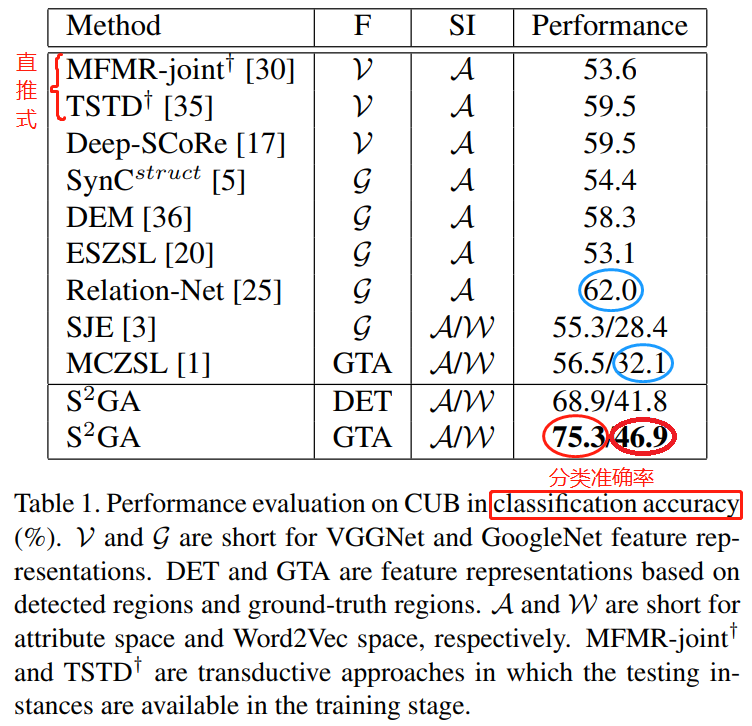
实验分析:论文方法和[1]用的是局部特征,其他方法用的是全局特征。
实验2——相同设置对比实验,CUB+NABird
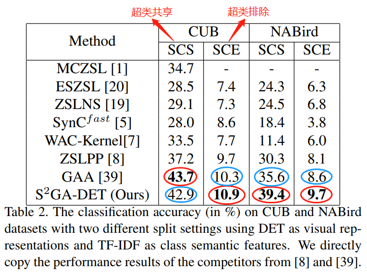
实验分析:SCE设置下,超类不共享,小类别之间的相关性最小,知识迁移更难,更具挑战,所以效果更差。
实验3:——语义空间对比实验,CUB
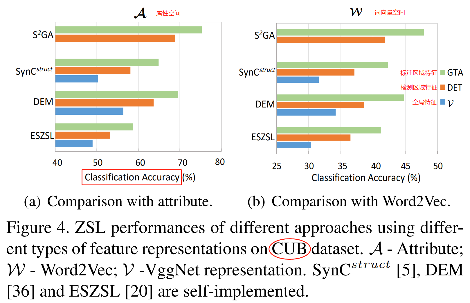
实验分析:
- 局部特征比全局特征更具有判别性
- 属性特征比词向量语义信息丰富
实验4——注意力实验,CUB+NABird
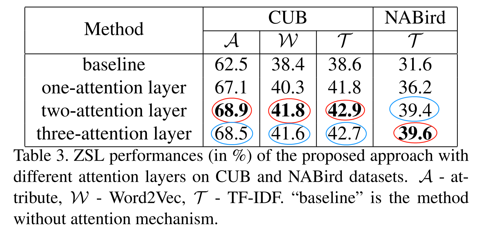
实验分析:两层注意力性能最高
实验5:——ZSL 检索,CUB+NABird
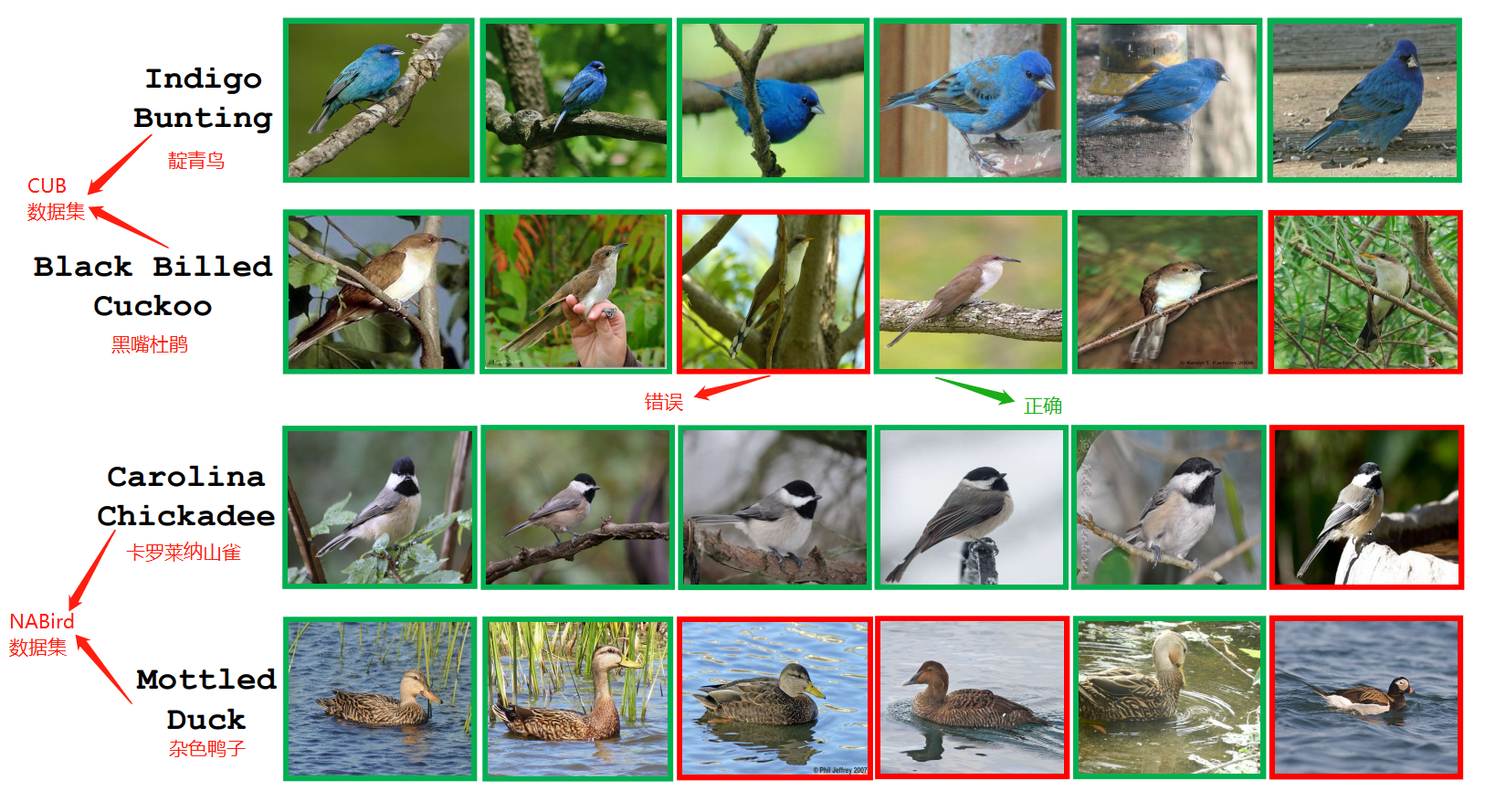
实验分析:
- 零样本检索的任务是:在未见类数据集中检索与未见类的指定类别语义描述相关的图像。
The task of zero-shot retrieval is to retrieve the relevant images from unseen class set related to the specified class semantic descriptions of unseen classes.- 检索任务的可视化结果发现,性能好的类别,他们的类内变化很微小;性能差的类别,他们的类间变化很小。
例如,
第一行,“靛青鸟”的前6个检索图像都来自标注类别;因为他们的视觉特征相似。
第二行,请求“黑嘴杜鹃”检索到一些实例来自它的姻亲“黄嘴杜鹃”,因为他们的视觉特征太像了没法区分。
总结
- 使用堆叠注意力,从表3看,注意力的收益是6.4%(CUB数据集)
问题1: 零样本学习中,有没有验证集?训练流程是怎样的?训练集阶段和测试阶段是怎么使用数据的?
1)没有,只有训练集和测试集。
2)先在训练集上进行训练模型,得到模型后直接在测试集上进行测试。
3)训练集被分为不同的batch,每次随机取batch然后训练模型,进行多次迭代;测试时对所有样本进行预测,计算精度。
问题2: seman和seman_pro区别?
seman–样本语义;seman_pro–类别语义。
2019/8/13
本文数据来自ZSL_PP_CVPR17,其中有CUB和NABird两个数据集的语料库语义(TF-IDF),本文对两个数据集TF-IDF进行了pca降维,分别降到200和400维。实验验证:在MATLAB 2017a,pca和princomp是有区别的,pca对CUB的数据返回的协方差矩阵只包含前199维,而princomp能返回所有维。
[c,s]=pca(PredicateMatrix);

[c,s]=princomp(PredicateMatrix);

参考:
- 西瓜书229
- 机器学习算法系列(22):主成分分析
收录经典的PCA代码(某大牛实现的):
PCA.m
function [eigvector, eigvalue] = PCA(data, options)
%PCA	Principal Component Analysis
%
%	Usage:
%       [eigvector, eigvalue] = PCA(data, options)
%       [eigvector, eigvalue] = PCA(data)
%
%             Input:
%               data       - Data matrix. Each row vector of fea is a data point.
%
%     options.ReducedDim   - The dimensionality of the reduced subspace. If 0,
%                         all the dimensions will be kept.
%                         Default is 0.
%
%             Output:
%               eigvector - Each column is an embedding function, for a new
%                           data point (row vector) x,  y = x*eigvector
%                           will be the embedding result of x.
%               eigvalue  - The sorted eigvalue of PCA eigen-problem.
%
%	Examples:
% 			fea = rand(7,10);
%           options=[];
%           options.ReducedDim=4;
% 			[eigvector,eigvalue] = PCA(fea,4);
%           Y = fea*eigvector;
%
%   version 3.0 --Dec/2011
%   version 2.2 --Feb/2009
%   version 2.1 --June/2007
%   version 2.0 --May/2007
%   version 1.1 --Feb/2006
%   version 1.0 --April/2004
%
%   Written by Deng Cai (dengcai AT gmail.com)
%

if (~exist('options','var'))
    options = [];
end

ReducedDim = 0;
if isfield(options,'ReducedDim')
    ReducedDim = options.ReducedDim;
end


[nSmp,nFea] = size(data);
if (ReducedDim > nFea) || (ReducedDim <=0)
    ReducedDim = nFea;
end


if issparse(data)
    data = full(data);
end
sampleMean = mean(data,1);
data = (data - repmat(sampleMean,nSmp,1));

[eigvector, eigvalue] = mySVD(data',ReducedDim);
eigvalue = full(diag(eigvalue)).^2;

if isfield(options,'PCARatio')
    sumEig = sum(eigvalue);
    sumEig = sumEig*options.PCARatio;
    sumNow = 0;
    for idx = 1:length(eigvalue)
        sumNow = sumNow + eigvalue(idx);
        if sumNow >= sumEig
            break;
        end
    end
    eigvector = eigvector(:,1:idx);
end
mySVD.m
function [U, S, V] = mySVD(X,ReducedDim)
%mySVD    Accelerated singular value decomposition.
%   [U,S,V] = mySVD(X) produces a diagonal matrix S, of the
%   dimension as the rank of X and with nonnegative diagonal elements in
%   decreasing order, and unitary matrices U and V so that
%   X = U*S*V'.
%
%   [U,S,V] = mySVD(X,ReducedDim) produces a diagonal matrix S, of the
%   dimension as ReducedDim and with nonnegative diagonal elements in
%   decreasing order, and unitary matrices U and V so that
%   Xhat = U*S*V' is the best approximation (with respect to F norm) of X
%   among all the matrices with rank no larger than ReducedDim.
%
%   Based on the size of X, mySVD computes the eigvectors of X*X^T or X^T*X
%   first, and then convert them to the eigenvectors of the other.
%
%   See also SVD.
%
%   version 2.0 --Feb/2009
%   version 1.0 --April/2004
%
%   Written by Deng Cai (dengcai AT gmail.com)
%

MAX_MATRIX_SIZE = 1600; % You can change this number according your machine computational power
EIGVECTOR_RATIO = 0.1; % You can change this number according your machine computational power


if ~exist('ReducedDim','var')
    ReducedDim = 0;
end

[nSmp, mFea] = size(X);
if mFea/nSmp > 1.0713
    ddata = X*X';
    ddata = max(ddata,ddata');

    dimMatrix = size(ddata,1);
    if (ReducedDim > 0) && (dimMatrix > MAX_MATRIX_SIZE) && (ReducedDim < dimMatrix*EIGVECTOR_RATIO)
        option = struct('disp',0);
        [U, eigvalue] = eigs(ddata,ReducedDim,'la',option);
        eigvalue = diag(eigvalue);
    else
        if issparse(ddata)
            ddata = full(ddata);
        end

        [U, eigvalue] = eig(ddata);
        eigvalue = diag(eigvalue);
        [dump, index] = sort(-eigvalue);
        eigvalue = eigvalue(index);
        U = U(:, index);
    end
    clear ddata;

    maxEigValue = max(abs(eigvalue));
    eigIdx = find(abs(eigvalue)/maxEigValue < 1e-10);
    eigvalue(eigIdx) = [];
    U(:,eigIdx) = [];

    if (ReducedDim > 0) && (ReducedDim < length(eigvalue))
        eigvalue = eigvalue(1:ReducedDim);
        U = U(:,1:ReducedDim);
    end

    eigvalue_Half = eigvalue.^.5;
    S =  spdiags(eigvalue_Half,0,length(eigvalue_Half),length(eigvalue_Half));

    if nargout >= 3
        eigvalue_MinusHalf = eigvalue_Half.^-1;
        V = X'*(U.*repmat(eigvalue_MinusHalf',size(U,1),1));
    end
else
    ddata = X'*X;
    ddata = max(ddata,ddata');

    dimMatrix = size(ddata,1);
    if (ReducedDim > 0) && (dimMatrix > MAX_MATRIX_SIZE) && (ReducedDim < dimMatrix*EIGVECTOR_RATIO)
        option = struct('disp',0);
        [V, eigvalue] = eigs(ddata,ReducedDim,'la',option);
        eigvalue = diag(eigvalue);
    else
        if issparse(ddata)
            ddata = full(ddata);
        end

        [V, eigvalue] = eig(ddata);
        eigvalue = diag(eigvalue);

        [dump, index] = sort(-eigvalue);
        eigvalue = eigvalue(index);
        V = V(:, index);
    end
    clear ddata;

    maxEigValue = max(abs(eigvalue));
    eigIdx = find(abs(eigvalue)/maxEigValue < 1e-10);
    eigvalue(eigIdx) = [];
    V(:,eigIdx) = [];

    if (ReducedDim > 0) && (ReducedDim < length(eigvalue))
        eigvalue = eigvalue(1:ReducedDim);
        V = V(:,1:ReducedDim);
    end

    eigvalue_Half = eigvalue.^.5;
    S =  spdiags(eigvalue_Half,0,length(eigvalue_Half),length(eigvalue_Half));

    eigvalue_MinusHalf = eigvalue_Half.^-1;
    U = X*(V.*repmat(eigvalue_MinusHalf',size(V,1),1));
end
用这份代码的降维结果和本文提供的降维结果非常一致。


 336
336


 被折叠的 条评论
为什么被折叠?
被折叠的 条评论
为什么被折叠?
 到【灌水乐园】发言


