混合高斯模型比单高斯模型_从零开始实现的高斯混合模型

最新推荐文章于 2022-08-28 16:50:25 发布

weixin_26630173

最新推荐文章于 2022-08-28 16:50:25 发布

阅读量481

点赞数

文章标签：机器学习 python tensorflow 人工智能 nlp

原文链接：https://towardsdatascience.com/gaussian-mixture-models-implemented-from-scratch-1857e40ea566

版权

混合高斯模型比单高斯模型

From the rising of the Machine Learning and Artificial Intelligence fields Probability Theory was a powerful tool, that allowed us to handle uncertainty in a lot of applications, from classification to forecasting tasks. Today I would like to talk with you more about the use of Probability and Gaussian distribution in clustering problems, implementing on the way the GMM model. So let’s get started

随着机器学习和人工智能领域的兴起，概率论是一种强大的工具，它使我们能够处理从分类到预测任务的许多应用程序中的不确定性。今天，我想与您更多地谈谈在GMM模型中实施概率和高斯分布在聚类问题中的应用。所以我们开始吧

什么是GMM？ (What is GMM?)

GMM (or Gaussian Mixture Models) is an algorithm that using the estimation of the density of the dataset to split the dataset in a preliminary defined number of clusters. For a better understandability, I will explain in parallel the theory and will show the code for implementing it.

GMM(或高斯混合模型)是一种算法，它使用数据集密度的估计将数据集划分为初步定义的数量的聚类。为了更好地理解，我将并行解释该理论并显示实现该理论的代码。

For this implementation, I will use the EM (Expectation-Maximization) algorithm.

对于此实现，我将使用EM(期望最大化)算法。

理论和代码是最好的组合。 (The theory and the code is the best combination.)

Firstly let’s import all needed libraries:

首先，让我们导入所有需要的库：

import numpy as np
import pandas as pd

I highly recommend following the standards of sci-kit learn library when implementing a model on your own. That’s why we will implement GMM as a class. Let’s also the __init_function.

我强烈建议您自己实施模型时，遵循sci-kit学习库的标准。这就是为什么我们将GMM实施为类。让我们还有__init_function。

class GMM:
    def __init__(self, n_components, max_iter = 100, comp_names=None):
        self.n_componets = n_components
        self.max_iter = max_iter
        if comp_names == None:
            self.comp_names = [f"comp{index}" for index in range(self.n_componets)]
        else:
            self.comp_names = comp_names
        # pi list contains the fraction of the dataset for every cluster
        self.pi = [1/self.n_componets for comp in range(self.n_componets)]

Shortly saying, n_components is the number of cluster in which whe want to split our data. max_iter represents the number of interations taken by the algorithm and comp_names is a list of string with n_components number of elements, that are interpreted as names of clusters.

简而言之 ， n_components是要在其中拆分数据的群集的数量。 max_iter表示算法进行的交互次数，comp_names是具有n_components个元素数量的字符串的列表，这些元素被解释为簇的名称。

拟合功能。 (The fit function.)

So before we get to the EM-algorithm we must split our dataset. after that, we must initiate 2 lists. One list containing the mean vectors (each element of the vector is the mean of columns) for every subset. The second list is containing the covariance matrix of each subset.

因此，在进入EM算法之前，必须先拆分数据集。之后，我们必须启动2个列表。每个子集包含一个均值向量的列表(向量的每个元素是列的均值)。第二个列表包含每个子集的协方差矩阵。

def fit(self, X):
        # Spliting the data in n_componets sub-sets
        new_X = np.array_split(X, self.n_componets)
        # Initial computation of the mean-vector and covarience matrix
        self.mean_vector = [np.mean(x, axis=0) for x in new_X]
        self.covariance_matrixes = [np.cov(x.T) for x in new_X]
        # Deleting the new_X matrix because we will not need it anymore
        del new_X

Now we can get to EM-algorithm.

现在我们可以进入EM算法。

EM算法。 (EM-algorithm.)

As the name says the EM-algorithm is divided in 2 steps — E and M.

顾名思义，EM算法分为两个步骤-E和M。

电子步骤： (E-step:)

During the Estimation step, we calculate the r matrix. It is calculated using the formula below.

在估计步骤中，我们计算r矩阵。使用以下公式计算。

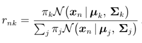
Image for post — The formula for calucalting the r (resposnsabilities) matrix (source — Mathemathis for Machine Learning Book)

r matrix is also known as ‘responsibilities’ and can be interpreted in the following way. Rows are the samples from the dataset, while columns represent every cluster, the elements of this matrix are interpreted as follows rnk is the probability of sample n to be part of cluster k. When the algorithm will converge we will use this matrix to predict the points cluster.

r矩阵也称为“责任” ，可以按以下方式解释。行是数据集中的样本，而列表示每个聚类，该矩阵的元素解释如下：rnk是样本n成为聚类k的一部分的概率。当算法收敛时，我们将使用此矩阵来预测点簇。

Also, we calculate the N list, in which each element is basically the sum of the correspondent column in the r matrix. The following code is doing that.

同样，我们计算N列表，其中每个元素基本上是r矩阵中对应列的总和。下面的代码正在执行此操作。

for iteration in range(self.max_iter):
    ''' ----------------   E - STEP   ------------------ '''
    # Initiating the r matrix, evrey row contains the probabilities
    # for every cluster for this row
    self.r = np.zeros((len(X), self.n_componets))
    # Calculating the r matrix
    for n in range(len(X)):
        for k in range(self.n_componets):
            self.r[n][k] = self.pi[k] * self.multivariate_normal(X[n], self.mean_vector[k], self.covariance_matrixes[k])
            self.r[n][k] /= sum([self.pi[j]*self.multivariate_normal(X[n], self.mean_vector[j], self.covariance_matrixes[j]) for j in range(self.n_componets)])
    # Calculating the N
    N = np.sum(self.r, axis=0)

Point that the multivariate_normal is just the formular for normal distribution applyed to vectors, it is used to calculate the probability for vectors in a normal sitribution.

指出multivariate_normal只是应用于向量的正态分布的公式，它用于计算正态分布中向量的概率。

and the code bellow implement it, taking the row vector, mean vector and the covariance matrix.

然后由下面的代码实现，它采用行向量，均值向量和协方差矩阵。

def multivariate_normal(self, X, mean_vector, covariance_matrix):
    return (2*np.pi)**(-len(X)/2)*np.linalg.det(covariance_matrix)**(-1/2)*np.exp(-np.dot(np.dot((X-mean_vector).T, np.linalg.inv(covariance_matrix)), (X-mean_vector))/2)

Looks a little bit messy but, you can find the full code there.

看起来有点混乱，但是您可以在此处找到完整的代码。

M步： (M-step:)

During the Maximization-step we will step-by-step set the value fo the mean vectors and covariance matrices to describe with them the clusters. To do that we will use the following formulas.

在最大化步骤中，我们将逐步设置均值向量和协方差矩阵的值，以用它们描述聚类。为此，我们将使用以下公式。

In the code I will like that:

在代码中，我会这样：

''' ---------------   M - STEP   --------------- '''
# Initializing the mean vector as a zero vector
self.mean_vector = np.zeros((self.n_componets, len(X[0])))
# Updating the mean vector
for k in range(self.n_componets):
    for n in range(len(X)):
        self.mean_vector[k] += self.r[n][k] * X[n]
        self.mean_vector = [1/N[k]*self.mean_vector[k] for k in range(self.n_componets)]
# Initiating the list of the covariance matrixes
self.covariance_matrixes = [np.zeros((len(X[0]), len(X[0]))) for k in range(self.n_componets)]
# Updating the covariance matrices
for k in range(self.n_componets):
    self.covariance_matrixes[k] = np.cov(X.T, aweights=(self.r[:, k]), ddof=0)
self.covariance_matrixes = [1/N[k]*self.covariance_matrixes[k] for k in range(self.n_componets)]
# Updating the pi list
self.pi = [N[k]/len(X) for k in range(self.n_componets)]

And we are done with fit function. Etiratively applying EM-algorithm will make the GMM fianlly to converge.

我们已经完成了拟合功能。合理地应用EM算法将使GMM最终收敛。

预测功能。 (The predict function.)

The predict function is actually very simple we simply use the multivariate normal function using the optimal mean vectors and covariance matrices for each cluster, to find using which gives the biggest values.

预测函数实际上非常简单，我们简单地使用多元正态函数，对每个聚类使用最佳均值向量和协方差矩阵，以找出具有最大价值的函数。

def predict(self, X):
        probas = []
        for n in range(len(X)):
            probas.append([self.multivariate_normal(X[n], self.mean_vector[k], self.covariance_matrixes[k])
                           for k in range(self.n_componets)])
        cluster = []
        for proba in probas:
            cluster.append(self.comp_names[proba.index(max(proba))])
        return cluster

结果。 (The result.)

To test the model I chose to compare it with the GMM implemented in the sci-kit library. I generated 2 datasets using sci-kit learn dataset generating function — make_blobs with different setings. So that is the result.

为了测试模型，我选择将其与sci-kit库中实现的GMM进行比较。我使用sci-kit Learn数据集生成功能-具有不同设置的make_blobs生成了2个数据集。这就是结果。

The clustering of our model and the sci-kit one are almost identical. A good result. The full code you can find there.

我们的模型和sci-kit的聚类几乎相同。好结果您可以在此处找到完整的代码。

This article was made with ❤ by Sigmoid.

本文由Sigmoid使用❤撰写。

Useful links:

有用的链接：

https://github.com/ScienceKot/mysklearn/tree/master/Gaussian%20Mixture%20Models
https://github.com/ScienceKot/mysklearn/tree/master/Gaussian%20Mixture%20Models
https://en.wikipedia.org/wiki/Expectation%E2%80%93maximization_algorithm
https://zh.wikipedia.org/wiki/期望％E2％80％93maximization_algorithm
Mathematics for Machine Learning by Cheng Soon Ong, Marc Peter Deisenroth and A. Aldo Faisal
郑顺(Ong Soon Ong)，马克·彼得·德森罗特(Marc Peter Deisenroth)和A.

翻译自: https://towardsdatascience.com/gaussian-mixture-models-implemented-from-scratch-1857e40ea566

混合高斯模型比单高斯模型

weixin_26630173

关注

0
点赞
踩
1

收藏

觉得还不错? 一键收藏
0
评论
混合高斯模型比单高斯模型_从零开始实现的高斯混合模型

混合高斯模型比单高斯模型From the rising of the Machine Learning and Artificial Intelligence fields Probability Theory was a powerful tool, that allowed us to handle uncertainty in a lot of applications, from clas...
复制链接

扫一扫