单层rnn和多层rnn_使用rnn进行pos标记

最新推荐文章于 2023-06-13 23:57:56 发布

weixin_26630173

最新推荐文章于 2023-06-13 23:57:56 发布

阅读量936

点赞数

文章标签： python java

原文链接：https://towardsdatascience.com/pos-tagging-using-rnn-7f08a522f849

版权

单层rnn和多层rnn

The classical way of doing POS tagging is using some variant of Hidden Markov Model. Here we'll see how we could do that using Recurrent neural networks. The original RNN architecture has some variants too. It has a novel RNN architecture — the Bidirectional RNN which is capable of reading sequences in the ‘reverse order’ as well and has proven to boost performance significantly.

进行POS标签的经典方法是使用“ 隐马尔可夫模型”的某些变体。在这里，我们将看到如何使用递归神经网络来做到这一点。原始的RNN架构也有一些变体。它具有新颖的RNN架构- 双向RNN ，它也能够以“逆序”读取序列，并已证明可以显着提高性能。

Then two important cutting-edge variants of the RNN which have made it possible to train large networks on real datasets. Although RNNs are capable of solving a variety of sequence problems, their architecture itself is their biggest enemy due to the problems of exploding and vanishing gradients that occur during the training of RNNs. This problem is solved by two popular gated RNN architectures — the Long, Short Term Memory (LSTM) and the Gated Recurrent Unit (GRU). We’ll look into all these models here with respect to POS tagging.

然后是RNN的两个重要的前沿变体，使在实际数据集上训练大型网络成为可能。尽管RNN能够解决各种序列问题，但是由于RNN训练过程中出现的爆炸和消失梯度问题，其架构本身是其最大的敌人。此问题由两种流行的门控RNN架构解决- 长期，短期内存(LSTM)和门控循环单元(GRU)。 我们将在这里针对POS标记研究所有这些模型。

POS标记—概述 (POS Tagging — An Overview)

The process of classifying words into their parts of speech and labeling them accordingly is known as part-of-speech tagging, or simply POS-tagging. The NLTK library has a number of corpora that contain words and their POS tag. I will be using the POS tagged corpora i.e treebank, conll2000, and brown from NLTK to demonstrate the key concepts. To get into the codes directly, an accompanying notebook is published on Kaggle.

将单词分类为语音部分并对其进行相应标记的过程称为词性标记 ，或简称为POS标记 。 NLTK库具有许多包含单词及其POS标签的语料库。我将使用POS标记语料库即树库 ，conll2000，和棕色从NLTK证明的关键概念。为了直接进入代码，在Kaggle上发布了一个随附的笔记本。

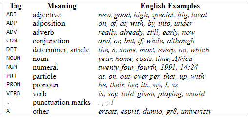
The following table provides information about some of the major tags:

下表提供有关一些主要标签的信息：

Image for post — **POS-tagging** **POS标签**

文章布局 (Article Layout)

Preprocess data
预处理数据
Word Embeddings
词嵌入
Vanilla RNN
香草RNN
LSTM
LSTM
GRU
格鲁
Bidirectional LSTM
双向LSTM
Model Evaluation
模型评估

导入数据集 (Importing the dataset)

Let’s begin with importing the necessary libraries and loading the dataset. This is a requisite step in every data analysis process(The complete code can be viewed here). We’ll be loading the data first using three well-known text corpora and taking the union of those.

让我们从导入必要的库并加载数据集开始。这是每个数据分析过程中必不可少的步骤(可以在此处查看完整的代码)。我们将首先使用三个著名的文本语料库加载数据，然后将它们合并。

# Importing and Loading the data into data frame
# load POS tagged corpora from NLTK
treebank_corpus = treebank.tagged_sents(tagset='universal')
brown_corpus = brown.tagged_sents(tagset='universal')
conll_corpus = conll2000.tagged_sents(tagset='universal')# Merging the dataframes to create a master dftagged_sentences = treebank_corpus + brown_corpus + conll_corpus

1.预处理数据 (1. Preprocess data)

As a part of preprocessing, we’ll be performing various steps such as dividing data into words and tags, Vectorise X and Y, and Pad sequences.

作为预处理的一部分，我们将执行各种步骤，例如将数据分为单词和标签，Vectorise X和Y以及Pad序列。

Let's look at the data first. For each of the words below, there is a tag associated with it.

让我们先来看数据。对于下面的每个单词，都有一个与之关联的标签。

# let's look at the data
tagged_sentences[7]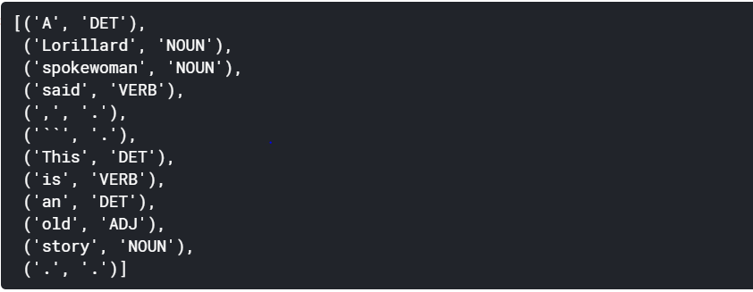

将数据分为单词(X)和标签(Y) (Divide data in words (X) and tags (Y))

Since this is a many-to-many problem, each data point will be a different sentence of the corpora. Each data point will have multiple words in the input sequence. This is what we will refer to as X. Each word will have its corresponding tag in the output sequence. This what we will refer to as Y. Sample dataset:

由于这是一个多对多的问题，因此每个数据点将是语料库的不同句子。每个数据点在输入序列中将有多个单词。这就是我们所说的X。每个单词在输出序列中都有其相应的标签。这就是我们所说的Y。样本数据集：

X = [] # store input sequence
Y = [] # store output sequencefor sentence in tagged_sentences:
 X_sentence = []
 Y_sentence = []
 for entity in sentence: 
 X_sentence.append(entity[0]) # entity[0] contains the word
 Y_sentence.append(entity[1]) # entity[1] contains corresponding tag
 X.append(X_sentence)
 Y.append(Y_sentence)num_words = len(set([word.lower() for sentence in X for word in sentence]))
num_tags   = len(set([word.lower() for sentence in Y for word in sentence]))print("Total number of tagged sentences: {}".format(len(X)))
print("Vocabulary size: {}".format(num_words))
print("Total number of tags: {}".format(num_tags))

# let’s look at first data point
# this is one data point that will be fed to the RNN
print(‘sample X: ‘, X[0], ‘\n’)
print(‘sample Y: ‘, Y[0], ‘\n’)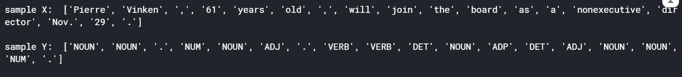

# In this many-to-many problem, the length of each input and output sequence must be the same.
# Since each word is tagged, it’s important to make sure that the length of input sequence equals the output sequenceprint(“Length of first input sequence : {}”.format(len(X[0])))
print(“Length of first output sequence : {}”.format(len(Y[0])))

The next thing we need to figure out is how are we going to feed these inputs to an RNN. If we have to give the words as input to any neural networks then we essentially have to convert them into numbers. We need to create a word embedding or one-hot vectors i.e. a vector of numbers form of each word. To start with this we'll first encode the input and output which will give a blind unique id to each word in the entire corpus for input data. On the other hand, we have the Y matrix(tags/output data). We have twelve POS tags here, treating each of them as a class and each pos tag is converted into one-hot encoding of length twelve. We’ll use the Tokenizer() function from Keras library to encode text sequence to integer sequence.

接下来需要弄清楚的是如何将这些输入馈送到RNN。如果我们必须将单词作为任何神经网络的输入，那么我们就必须将它们转换为数字。我们需要创建一个词嵌入或单词向量，即每个词的数字形式的向量。首先，我们将首先对输入和输出进行编码，这将为整个语料库中的每个单词的输入数据提供一个盲目的唯一ID。另一方面，我们有Y矩阵(标签/输出数据)。我们这里有十二个POS标签，将每个POS标签视为一个类，并且每个pos标签都转换为长度为十二的一键编码。我们将使用Keras库中的Tokenizer()函数将文本序列编码为整数序列。

向量化X和Y (Vectorise X and Y)

# encode Xword_tokenizer = Tokenizer()              # instantiate tokeniser
word_tokenizer.fit_on_texts(X)            # fit tokeniser on data# use the tokeniser to encode input sequence
X_encoded = word_tokenizer.texts_to_sequences(X)  # encode Ytag_tokenizer = Tokenizer()
tag_tokenizer.fit_on_texts(Y)
Y_encoded = tag_tokenizer.texts_to_sequences(Y)# look at first encoded data pointprint("** Raw data point **", "\n", "-"*100, "\n")
print('X: ', X[0], '\n')
print('Y: ', Y[0], '\n')
print()
print("** Encoded data point **", "\n", "-"*100, "\n")
print('X: ', X_encoded[0], '\n')
print('Y: ', Y_encoded[0], '\n')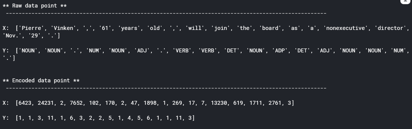

Make sure that each sequence of input and output is of the same length.

确保每个输入和输出序列具有相同的长度。

填充顺序 (Pad sequences)

The sentences in the corpus are not of the same length. Before we feed the input in the RNN model we need to fix the length of the sentences. We cannot dynamically allocate memory required to process each sentence in the corpus as they are of different lengths. Therefore the next step after encoding the data is to define the sequence lengths. We need to either pad short sentences or truncate long sentences to a fixed length. This fixed length, however, is a hyperparameter.

语料库中的句子长度不同。在将输入输入RNN模型之前，我们需要确定句子的长度。我们无法动态分配处理语料库中每个句子的长度所需的内存。因此，编码数据后的下一步是定义序列长度 。我们需要填充短句子或将长句子截断为固定长度。但是，此固定长度是超参数 。

# Pad each sequence to MAX_SEQ_LENGTH using KERAS’ pad_sequences() function. 
# Sentences longer than MAX_SEQ_LENGTH are truncated.
# Sentences shorter than MAX_SEQ_LENGTH are padded with zeroes.# Truncation and padding can either be ‘pre’ or ‘post’. 
# For padding we are using ‘pre’ padding type, that is, add zeroes on the left side.
# For truncation, we are using ‘post’, that is, truncate a sentence from right side.# sequences greater than 100 in length will be truncatedMAX_SEQ_LENGTH = 100X_padded = pad_sequences(X_encoded, maxlen=MAX_SEQ_LENGTH, padding=”pre”, truncating=”post”)
Y_padded = pad_sequences(Y_encoded, maxlen=MAX_SEQ_LENGTH, padding=”pre”, truncating=”post”)# print the first sequence
print(X_padded[0], "\n"*3)
print(Y_padded[0])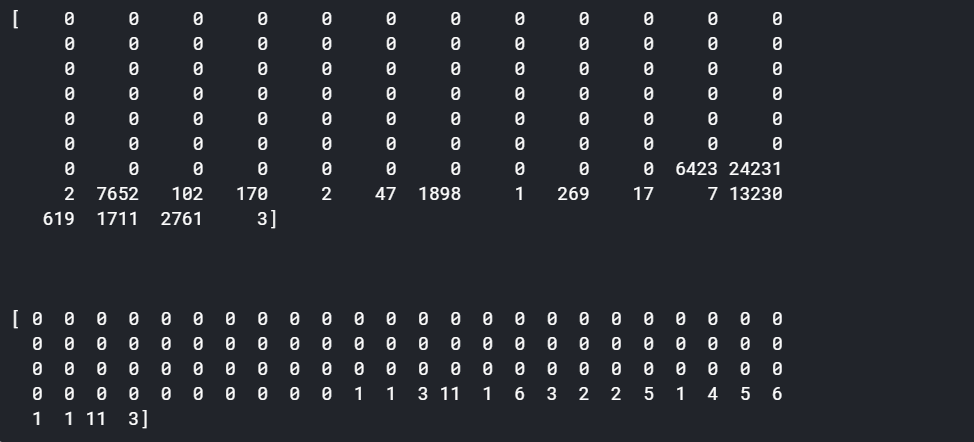

2.词嵌入 (2. Word embeddings)

You know that a better way (than one-hot vectors) to represent text is word embeddings. Currently, each word and each tag is encoded as an integer. We’ll use a more sophisticated technique to represent the input words (X) using what’s known as word embeddings.

您知道，一种更好的表示文本的方法(比单热向量)是单词嵌入 。当前，每个单词和每个标签被编码为整数。我们将使用一种更复杂的技术，通过所谓的词嵌入来表示输入词(X)。

However, to represent each tag in Y, we’ll simply use one-hot encoding scheme since there are only 12 tags in the dataset and the LSTM will have no problems in learning its own representation of these tags.

但是，为了表示Y中的每个标签，我们将仅使用单热编码方案，因为数据集中只有12个标签，并且LSTM在学习自己的这些标签表示时不会有问题。

To use word embeddings, you can go for either of the following models:

要使用单词嵌入，可以使用以下任一模型：

We’re using the word2vec model for no particular reason. Both of these are very efficient in representing words. You can try both and see which one works better.

出于特殊原因，我们正在使用word2vec模型。两者都非常有效地表示单词。您可以尝试两者，看看哪一个更好。

The dimension of a word embedding is: (VOCABULARY_SIZE, EMBEDDING_DIMENSION)

单词嵌入的维数为：(VOCABULARY_SIZE，EMBEDDING_DIMENSION)

将单词嵌入用于输入序列(X) (Use word embeddings for input sequences (X))

# word2vecpath = ‘../input/wordembeddings/GoogleNews-vectors-negative300.bin’# load word2vec using the following function present in the gensim library
word2vec = KeyedVectors.load_word2vec_format(path, binary=True)# assign word vectors from word2vec model
# each word in word2vec model is represented using a 300 dimensional vectorEMBEDDING_SIZE  = 300  
VOCABULARY_SIZE = len(word_tokenizer.word_index) + 1# create an empty embedding matix
embedding_weights = np.zeros((VOCABULARY_SIZE, EMBEDDING_SIZE))# create a word to index dictionary mapping
word2id = word_tokenizer.word_index# copy vectors from word2vec model to the words present in corpus
for word, index in word2id.items():
    try:
        embedding_weights[index, :] = word2vec[word]
    except KeyError:
        pass

对输出序列使用一键编码(Y) (Use one-hot encoding for output sequences (Y))

# use Keras’ to_categorical function to one-hot encode Y
Y = to_categorical(Y)

All the data preprocessing is now complete. Let’s now jump to the modeling part by splitting the data to train, validation, and test sets.

现在所有数据预处理已完成。现在，通过将数据拆分为训练，验证和测试集跳到建模部分。

Before using RNN, we must make sure the dimensions of the data are what an RNN expects. In general, an RNN expects the following shape

在使用RNN之前，我们必须确保数据的尺寸符合RNN的期望。通常，RNN期望以下形状

Shape of X: (#samples, #timesteps, #features)

X的形状：(＃samples，＃timesteps，＃features)

Shape of Y: (#samples, #timesteps, #features)

Y的形状：(＃samples，＃timesteps，＃features)

Now, there can be various variations in the shape that you use to feed an RNN depending on the type of architecture. Since the problem we’re working on has a many-to-many architecture, the input and the output both include number of timesteps which is nothing but the sequence length. But notice that the tensor X doesn’t have the third dimension, that is, number of features. That’s because we’re going to use word embeddings before feeding in the data to an RNN, and hence there is no need to explicitly mention the third dimension. That’s because when you use the Embedding() layer in Keras, the training data will automatically be converted to (#samples, #timesteps, #features) where #features will be the embedding dimension (and note that the Embedding layer is always the very first layer of an RNN). While using the embedding layer we only need to reshape the data to (#samples, #timesteps) which is what we have done. However, note that you’ll need to shape it to (#samples, #timesteps, #features) in case you don’t use the Embedding() layer in Keras.

现在，根据体系结构的类型，用于馈送RNN的形状可以有多种变化。由于我们正在处理的问题具有多对多的体系结构，因此输入和输出都包含时间步长，而这仅是序列长度。但是请注意，张量X没有第三维，即特征数量。这是因为在将数据输入到RNN之前，我们将使用词嵌入，因此无需明确提及第三维。那是因为当您在Keras中使用Embedding()层时，训练数据将自动转换为( #samples，#timesteps，#features )，其中#features将是嵌入维度(并且请注意，Embedding层始终是RNN的第一层)。使用嵌入层时，我们只需要将数据重塑为(#samples，#timesteps)，这就是我们所做的。但是，请注意，如果不在Keras中使用Embedding()层，则需要将其成形为(＃samples，＃timesteps，＃features)。

3. Vanilla RNN (3. Vanilla RNN)

Next, let’s build the RNN model. We’re going to use word embeddings to represent the words. Now, while training the model, you can also train the word embeddings along with the network weights. These are often called the embedding weights. While training, the embedding weights will be treated as normal weights of the network which are updated in each iteration.

接下来，让我们构建RNN模型。我们将使用单词嵌入来表示单词。现在，在训练模型的同时，您还可以训练单词嵌入以及网络权重。这些通常称为嵌入权重 。训练时，嵌入权重将被视为网络的正常权重，该权重在每次迭代中都会更新。

In the next few sections, we will try the following three RNN models:

在接下来的几节中，我们将尝试以下三种RNN模型：

RNN with arbitrarily initialized, untrainable embeddings: In this model, we will initialize the embedding weights arbitrarily. Further, we’ll freeze the embeddings, that is, we won’t allow the network to train them.
具有任意初始化且不可训练的嵌入的 RNN：在此模型中，我们将任意初始化嵌入权重。此外，我们将冻结嵌入 ，即我们将不允许网络对其进行训练。
RNN with arbitrarily initialized, trainable embeddings: In this model, we’ll allow the network to train the embeddings.
具有任意初始化的可训练嵌入的 RNN：在此模型中，我们将允许网络训练嵌入。
RNN with trainable word2vec embeddings: In this experiment, we’ll use word2vec word embeddings and also allow the network to train them further.
具有可训练word2vec嵌入的 RNN ：在本实验中，我们将使用word2vec词嵌入，还允许网络进一步训练它们。

未初始化的固定嵌入 (Uninitialized fixed embeddings)

Let’s start with the first experiment: a vanilla RNN with arbitrarily initialized, untrainable embedding. For this RNN we won’t use the pre-trained word embeddings. We’ll use randomly initialized embeddings. Moreover, we won’t update the embeddings weights.

让我们从第一个实验开始：具有任意初始化的，不可训练的嵌入的香草RNN 。对于此RNN，我们将不使用预训练的单词嵌入。我们将使用随机初始化的嵌入。此外，我们不会更新嵌入权重。

# create architecturernn_model = Sequential()# create embedding layer — usually the first layer in text problems
# vocabulary size — number of unique words in datarnn_model.add(Embedding(input_dim = VOCABULARY_SIZE, # length of vector with which each word is represented
 output_dim = EMBEDDING_SIZE, # length of input sequence
 input_length = MAX_SEQ_LENGTH, # False — don’t update the embeddings
 trainable = False 
))# add an RNN layer which contains 64 RNN cells
# True — return whole sequence; False — return single output of the end of the sequencernn_model.add(SimpleRNN(64, 
 return_sequences=True
))# add time distributed (output at each sequence) layer
rnn_model.add(TimeDistributed(Dense(NUM_CLASSES, activation=’softmax’)))#compile model
rnn_model.compile(loss      =  'categorical_crossentropy',
                  optimizer =  'adam',
                  metrics   =  ['acc'])# check summary of the model
rnn_model.summary()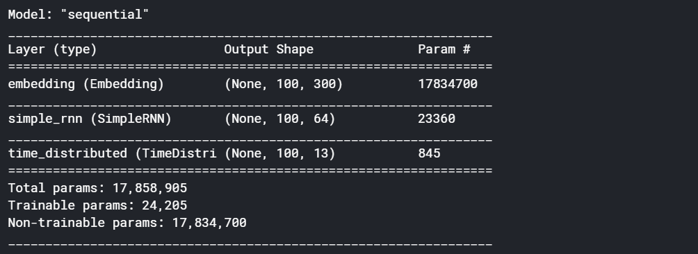

#fit model
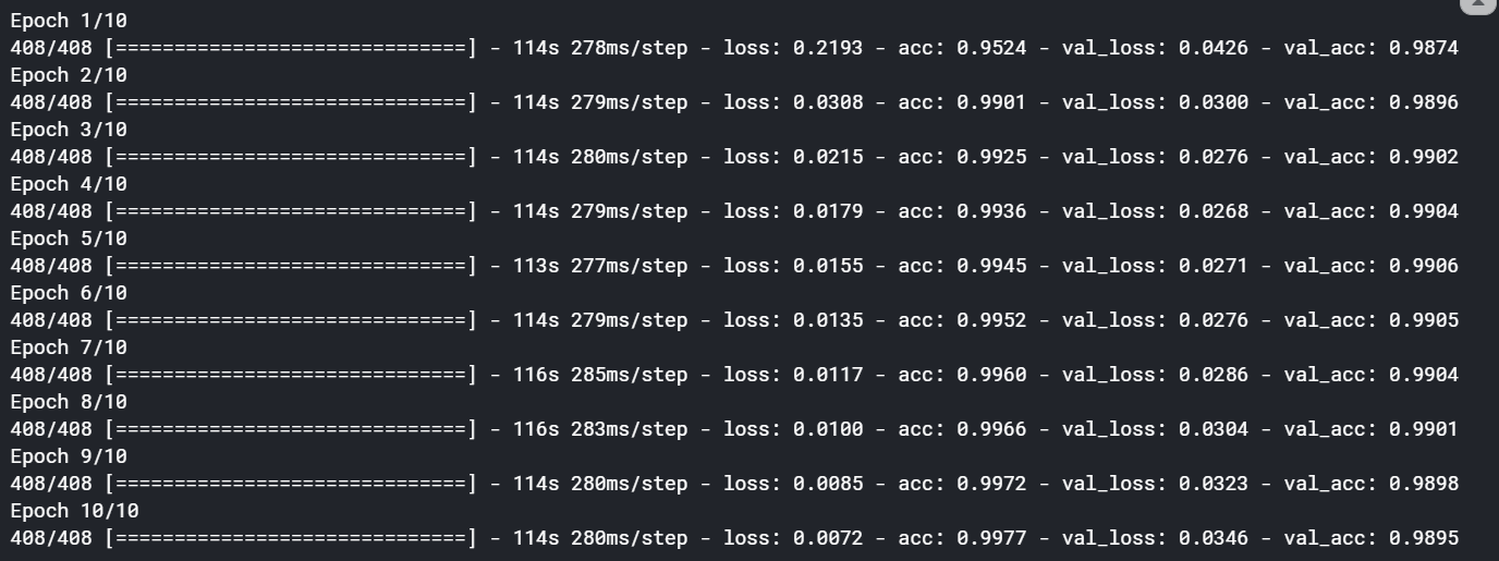
rnn_training = rnn_model.fit(X_train, Y_train, batch_size=128, epochs=10, validation_data=(X_validation, Y_validation))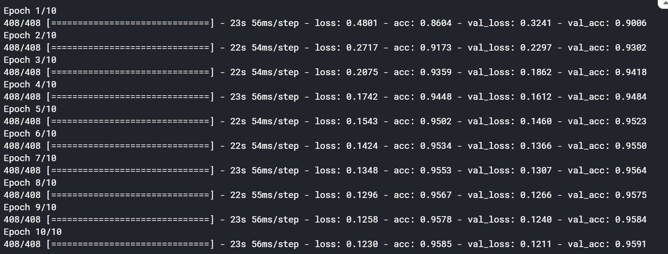

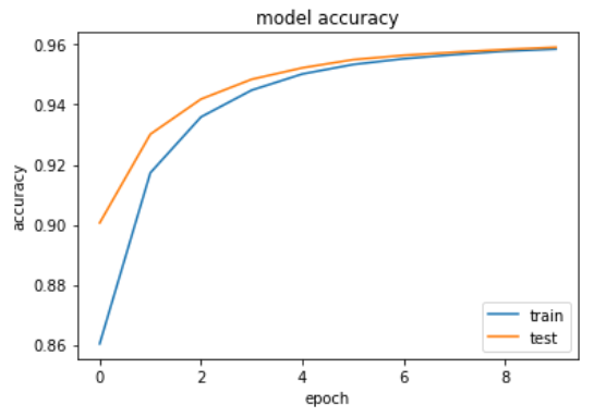
We can see here, after ten epoch, it is giving fairly decent accuracy of approx 95%. Also, we are getting a healthy growth curve below.

我们可以在这里看到，经过十个世纪之后，它给出了大约95％的相当不错的精度。 此外，我们在下面获得了健康的增长曲线。

未初始化的可训练嵌入 (Uninitialized trainable embeddings)

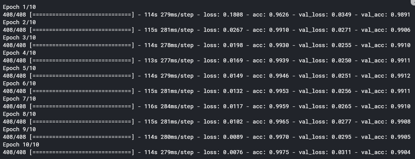
Next, try the second model — RNN with arbitrarily initialized, trainable embeddings. Here, we’ll allow the embeddings to get trained with the network. All I am doing is changing the parameter trainable to true i.e trainable = True. Rest all remains the same as above. On checking the model summary we can see that all the parameters have become trainable. i.e trainable params are equal to total params.

接下来，尝试第二种模型-具有任意初始化的可训练嵌入的 RNN。在这里，我们将允许嵌入知识通过网络进行训练。我正在做的就是将参数Trainable更改为true，即trainable = True。 其余所有与上述相同。在检查模型摘要时，我们可以看到所有参数均已变为可训练的。即，可训练参数等于总参数。

# check summary of the model
rnn_model.summary()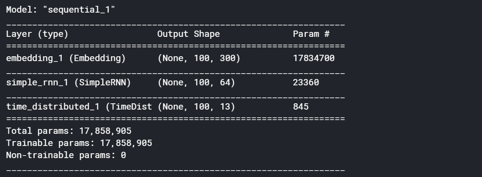

On fitting the model the accuracy has grown significantly. It has gone up to approx 98.95% by allowing the embedding weights to train. Therefore embedding has a significant effect on how the network is going to perform.

在拟合模型时，准确性显着提高。通过允许嵌入权重的训练，它已经上升到大约98.95％。因此，嵌入会对网络的运行方式产生重大影响。

we’ll now try the word2vec embeddings and see if that improves our model or not.

现在，我们将尝试使用word2vec嵌入，看看是否可以改善我们的模型。

使用预训练的嵌入权重 (Using pre-trained embedding weights)

Let’s now try the third experiment — RNN with trainable word2vec embeddings. Recall that we had loaded the word2vec embeddings in a matrix called ‘embedding_weights’. Using word2vec embeddings is just as easy as including this matrix in the model architecture.

现在让我们尝试第三个实验-具有可训练word2vec嵌入的 RNN 。回想一下，我们已将word2vec嵌入内容加载到名为“ embedding_weights”的矩阵中。使用word2vec嵌入就像在模型体系结构中包含此矩阵一样容易。

The network architecture is the same as above but instead of starting with an arbitrary embedding matrix, we’ll use pre-trained embedding weights (weights = [embedding_weights]) coming from word2vec. The accuracy, in this case, has gone even further to approx 99.04%.

网络架构与上述相同，但不是从任意的嵌入矩阵开始，而是使用来自word2vec的预训练嵌入权重( weights = [embedding_weights] )。在这种情况下，准确性甚至达到了约99.04％。

The results improved marginally in this case. That’s because the model was already performing very well. You’ll see much more improvements by using pre-trained embeddings in cases where you don’t have such a good model performance. Pre-trained embeddings provide a real boost in many applications.

在这种情况下，结果略有改善。那是因为模型已经表现出色。在模型性能不佳的情况下，通过使用预训练的嵌入，您将看到更多的改进。预训练的嵌入在许多应用中提供了真正的推动力。

4. LSTM (4. LSTM)

To solve the vanishing gradients problem, many attempts have been made to tweak the vanilla RNNs such that the gradients don’t die when sequences get long. The most popular and successful of these attempts has been the long, short-term memory network, or the LSTM. LSTMs have proven to be so effective that they have almost replaced vanilla RNNs.

为了解决消失的梯度问题，已经进行了许多尝试来调整香草RNN，以使梯度不会在序列变长时消失。这些尝试中最流行和最成功的是长期的短期内存网络或LSTM 。 LSTM已被证明是如此有效，以至于它们几乎取代了普通RNN。

Thus, one of the fundamental differences between an RNN and an LSTM is that an LSTM has an explicit memory unit which stores information relevant for learning some task. In the standard RNN, the only way the network remembers past information is through updating the hidden states over time, but it does not have an explicit memory to store information.

因此，RNN和LSTM之间的根本区别之一是LSTM具有显式的存储 单元，用于存储与学习某些任务相关的信息。在标准RNN中，网络记住过去信息的唯一方法是随着时间的推移更新隐藏状态，但是它没有显式的内存来存储信息。

On the other hand, in LSTMs, the memory units retain pieces of information even when the sequences get really long.

另一方面，在LSTM中，即使序列真的很长，存储单元也会保留信息。

Next, we’ll build an LSTM model instead of an RNN. We just need to replace the RNN layer with LSTM layer.

接下来，我们将构建LSTM模型而不是RNN。我们只需要用LSTM层替换RNN层即可。

# create architecturelstm_model = Sequential()# vocabulary size — number of unique words in data
# length of vector with which each word is representedlstm_model.add(Embedding(input_dim = VOCABULARY_SIZE, 
 output_dim = EMBEDDING_SIZE, # length of input sequenceinput_length = MAX_SEQ_LENGTH, # word embedding matrixweights = [embedding_weights],# True — update embeddings_weight matrixtrainable = True 
))# add an LSTM layer which contains 64 LSTM cells
# True — return whole sequence; False — return single output of the end of the sequence
lstm_model.add(LSTM(64, return_sequences=True))
lstm_model.add(TimeDistributed(Dense(NUM_CLASSES, activation=’softmax’)))#compile model
rnn_model.compile(loss      =  'categorical_crossentropy',
                  optimizer =  'adam',
                  metrics   =  ['acc'])# check summary of the model
rnn_model.summary()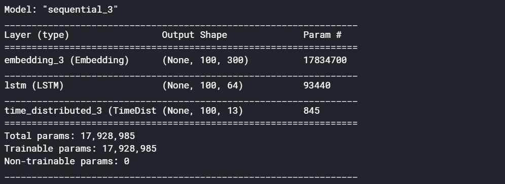

lstm_training = lstm_model.fit(X_train, Y_train, batch_size=128, epochs=10, validation_data=(X_validation, Y_validation))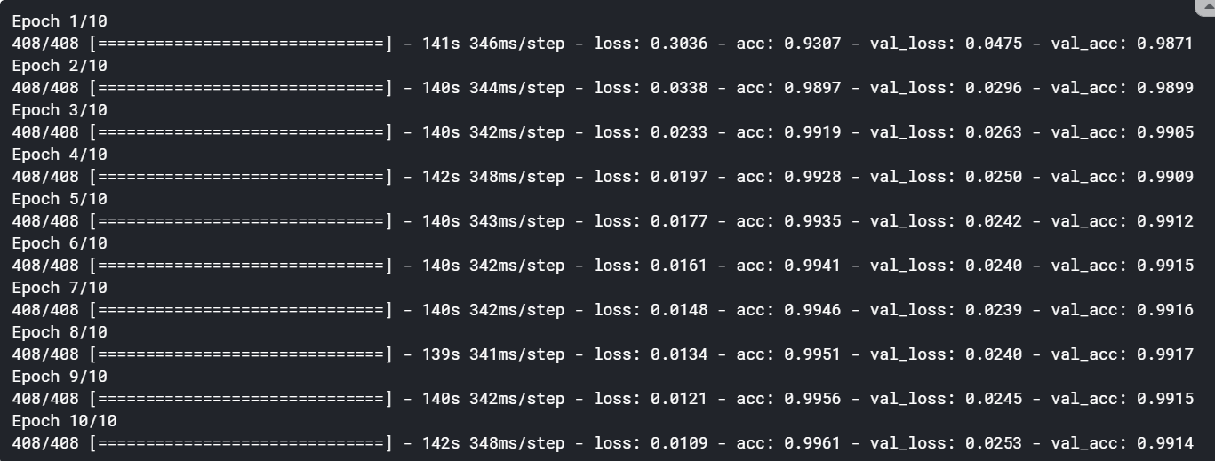

The LSTM model also provided some marginal improvement. However, if we use an LSTM model in other tasks such as language translation, image captioning, time series forecasting, etc. then you may see a significant boost in the performance.

LSTM模型也提供了一些改进。但是，如果我们在其他任务(例如语言翻译，图像字幕，时间序列预测等)中使用LSTM模型，则可能会看到性能的显着提高。

5. GRU (5. GRU)

Keeping in mind the computational expenses and the problem of overfitting, researchers have tried to come up with alternate structures of the LSTM cell. The most popular one of these alternatives is the gated recurrent unit (GRU). GRU being a simpler model than LSTM, it's always easier to train. LSTMs and GRUs have almost completely replaced the standard RNNs in practice because they’re more effective and faster to train than vanilla RNNs (despite the larger number of parameters).

考虑到计算费用和过度拟合的问题，研究人员试图提出LSTM单元的替代结构。这些替代方案中最流行的一种是门控循环单元(GRU)。 GRU是比LSTM更简单的模型，它总是容易训练。在实践中，LSTM和GRU几乎完全替代了标准RNN，因为它们比普通RNN更有效和更快地训练(尽管有大量参数)。

Let’s now build a GRU model. We’ll then also compare the performance of the RNN, LSTM, and the GRU model.

现在让我们建立一个GRU模型。然后，我们还将比较RNN，LSTM和GRU模型的性能。

# create architecturelstm_model = Sequential()# vocabulary size — number of unique words in data
# length of vector with which each word is representedlstm_model.add(Embedding(input_dim = VOCABULARY_SIZE, 
 output_dim = EMBEDDING_SIZE, # length of input sequenceinput_length = MAX_SEQ_LENGTH, # word embedding matrixweights = [embedding_weights],# True — update embeddings_weight matrixtrainable = True 
))# add an LSTM layer which contains 64 LSTM cells
# True — return whole sequence; False — return single output of the end of the sequence
lstm_model.add(GRU(64, return_sequences=True))
lstm_model.add(TimeDistributed(Dense(NUM_CLASSES, activation=’softmax’)))#compile model
rnn_model.compile(loss      =  'categorical_crossentropy',
                  optimizer =  'adam',
                  metrics   =  ['acc'])# check summary of the model
rnn_model.summary()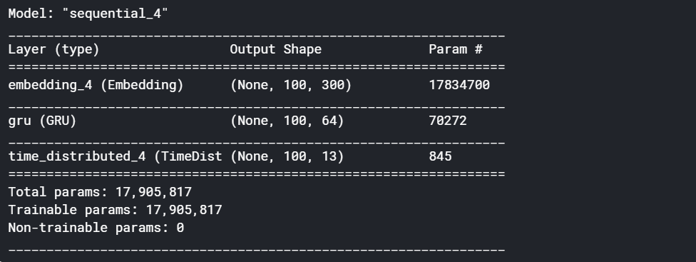

There is a reduction in params in GRU as compared to LSTM. Therefore we do get a significant boost in terms of computational efficiency with hardly any decremental effect in the performance of the model.

与LSTM相比，GRU中的参数有所减少。因此，我们在计算效率方面确实获得了显着提升，而模型性能几乎没有任何递减影响。

gru_training = gru_model.fit(X_train, Y_train, batch_size=128, epochs=10, validation_data=(X_validation, Y_validation))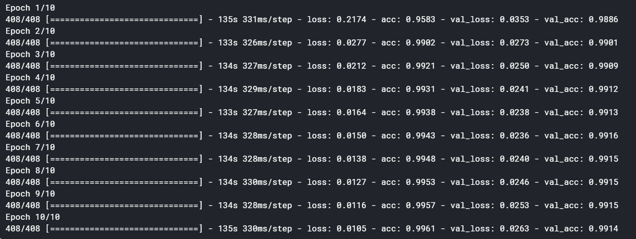

The accuracy of the model remains the same as the LSTM. But we saw that the time taken by an LSTM is greater than a GRU and an RNN. This was expected since the parameters in an LSTM and GRU are 4x and 3x of a normal RNN, respectively.

模型的准确性与LSTM相同。但是我们看到，LSTM花费的时间大于GRU和RNN花费的时间。这是可以预期的，因为LSTM和GRU中的参数分别是正常RNN的4倍和3倍。

6.双向LSTM (6. Bidirectional LSTM)

For example, when you want to assign a sentiment score to a piece of text (say a customer review), the network can see the entire review text before assigning them a score. On the other hand, in a task such as predicting the next word given previous few typed words, the network does not have access to the words in the future time steps while predicting the next word.

例如，当您要为一条文本分配一个情感分数 (例如客户评论)时，网络可以在为他们分配分数之前查看整个评论文本。另一方面，在诸如给定先前几个键入的单词的情况下预测下一个单词的任务中，网络在预测下一个单词时在将来的时间步中无法访问这些单词。

These two types of tasks are called offline and online sequence processing respectively.

这两种类型的任务分别称为离线和在线 序列处理 。

Now, there is a neat trick you can use with offline tasks — since the network has access to the entire sequence before making predictions, why not use this task to make the network ‘look at the future elements in the sequence’ while training, hoping that this will make the network learn better?

现在，您可以使用一个巧妙的技巧来处理脱机任务 -由于网络在进行预测之前可以访问整个序列，所以为什么不使用此任务使网络在训练时“查看序列中的未来元素”，希望这样可以使网络学习得更好？

This is the idea exploited by what is called bidirectional RNNs.

这就是所谓的双向RNN所利用的想法。

By using bidirectional RNNs, it is almost certain that you’ll get better results. However, bidirectional RNNs take almost double the time to train since the number of parameters of the network increase. Therefore, you have a tradeoff between training time and performance. The decision to use a bidirectional RNN depends on the computing resources that you have and the performance you are aiming for.

通过使用双向RNN，几乎可以肯定会获得更好的结果。然而，由于网络参数数量的增加，双向RNN花费几乎两倍的时间进行训练。因此，您需要在训练时间和性能之间进行权衡。使用双向RNN的决定取决于您拥有的计算资源和目标性能。

Finally, let’s build one more model — a bidirectional LSTM and compare its performance in terms of accuracy and training time as compared to the previous models.

最后，让我们建立另一个模型- 双向LSTM，并与以前的模型相比，在准确性和训练时间方面比较其性能。

# create architecturebidirect_model = Sequential()
bidirect_model.add(Embedding(input_dim = VOCABULARY_SIZE,
 output_dim = EMBEDDING_SIZE,
 input_length = MAX_SEQ_LENGTH,
 weights = [embedding_weights],
 trainable = True
))
bidirect_model.add(Bidirectional(LSTM(64, return_sequences=True)))
bidirect_model.add(TimeDistributed(Dense(NUM_CLASSES, activation=’softmax’)))#compile modelbidirect_model.compile(loss='categorical_crossentropy',
              optimizer='adam',
              metrics=['acc'])# check summary of model
bidirect_model.summary()

You can see the no of parameters has gone up. It does significantly shoot up the no of params.

您可以看到参数数量已经增加。它确实大大增加了参数数量。

bidirect_training = bidirect_model.fit(X_train, Y_train, batch_size=128, epochs=10, validation_data=(X_validation, Y_validation))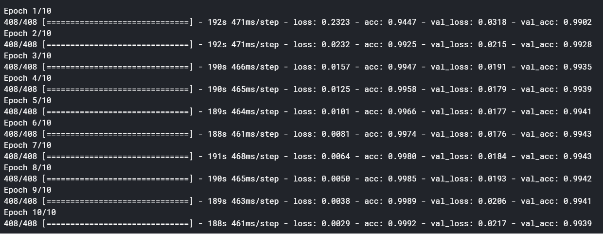

The bidirectional LSTM did increase the accuracy substantially (considering that the accuracy was already hitting the roof). This shows the power of bidirectional LSTMs. However, this increased accuracy comes at a cost. The time taken was almost double than of a normal LSTM network.

双向LSTM确实确实提高了准确性(考虑到准确性已经达到顶峰)。这显示了双向LSTM的强大功能。但是，这种提高的准确性是有代价的。所花费的时间几乎是普通LSTM网络的两倍。

7.模型评估 (7. Model evaluation)

Below is the quick summary of each of the four models we tried. We can see a trend here as we move from one model to another.

以下是我们尝试的四个模型的快速摘要。当我们从一种模型转移到另一种模型时，我们可以在这里看到趋势。

loss, accuracy = rnn_model.evaluate(X_test, Y_test, verbose = 1)
print(“Loss: {0},\nAccuracy: {1}”.format(loss, accuracy))

loss, accuracy = lstm_model.evaluate(X_test, Y_test, verbose = 1)
print(“Loss: {0},\nAccuracy: {1}”.format(loss, accuracy))

loss, accuracy = gru_model.evaluate(X_test, Y_test, verbose = 1)
print(“Loss: {0},\nAccuracy: {1}”.format(loss, accuracy))

loss, accuracy = bidirect_model.evaluate(X_test, Y_test, verbose = 1)
print("Loss: {0},\nAccuracy: {1}".format(loss, accuracy))

If you have any questions, recommendations, or critiques, I can be reached via LinkedIn or the comment section.

如果您有任何问题，建议或评论，可以通过LinkedIn或评论栏与我联系。

翻译自: https://towardsdatascience.com/pos-tagging-using-rnn-7f08a522f849

单层rnn和多层rnn

weixin_26630173

关注

0
点赞
踩
0

收藏

觉得还不错? 一键收藏
0
评论
单层rnn和多层rnn_使用rnn进行pos标记

单层rnn和多层rnnThe classical way of doing POS tagging is using some variant of Hidden Markov Model. Here we'll see how we could do that using Recurrent neural networks. The original RNN architecture has s...
复制链接

扫一扫