pca vc_vc高维pca和内核pca

最新推荐文章于 2021-10-12 19:26:52 发布

weixin_26632361

最新推荐文章于 2021-10-12 19:26:52 发布

阅读量111

点赞数

文章标签：内核

原文链接：https://medium.com/swlh/vc-high-dimensional-pca-and-kernel-pca-415ef47e2d15

版权

pca vc

This post assumes you already know what PCA is. If you don’t please check my previous post.

这篇文章假定您已经知道PCA是什么。如果您不这样做，请检查我以前的帖子。

n <p情况(高维PCA) (n < p case (High dimensional PCA))

If the feature space is bigger than the number of data points, our rank is determined by n-1 because it is centred by the mean. Therefore, the degree of freedom is reduced, we can calculate the last one by the previous n-1 data points because of the mean.

如果特征空间大于数据点的数量，则我们的排名由n-1确定，因为它的均值位于中心。因此，自由度降低了，由于均值，我们可以通过前n-1个数据点来计算最后一个。

We will use one fact to efficiently calculate the high dimensional PCA. All eigenvectors of S are in the span of z(the centred vector of the original data).

我们将使用一个事实来有效地计算高维PCA。 S的所有特征向量都在z的范围内(原始数据的中心向量)。

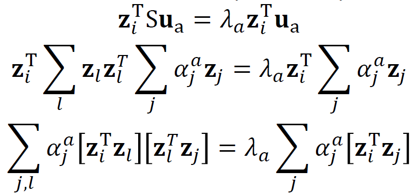
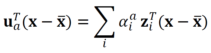
This proof starts with the eigenvalue decomposition of the scatter matrix. We can think of the inner product of S and u as the sum of vector inner products. We got u is some scalar product of z. The scalar coefficient consists of eigenvalue, eigenvector, and z transpose. We can reduce the computation with this fact from p x p eigenvalue problem to n x n eigenvalue problem.

该证明从散射矩阵的特征值分解开始。我们可以将S和u的内积视为向量内积的总和。我们得到u是z的标量积。标量系数由特征值，特征向量和z转置组成。利用这个事实，我们可以将计算从pxp特征值问题简化为nxn特征值问题。

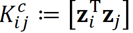
We start with the eigenvalue decomposition of the scatter matrix S and it becomes the eigenvalue decomposition of matrix K because its vector product is different, it is from the different index of the vectors. We assume the eigenvector of S is normalized and we easily calculate the alpha, this is what we want to get. The alpha is the coefficient of z spanning u.

我们从散布矩阵S的特征值分解开始，由于它的向量乘积不同(来自向量的不同索引)，因此它变为矩阵K的特征值分解。我们假设S的特征向量已归一化，我们很容易计算出alpha，这就是我们想要得到的。 alpha是z跨越u的系数。

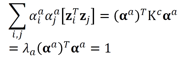
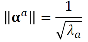
The dot product of u will be 1 and we can calculate the alpha with this fact as you can see above. The eigenvalue of K must be plus because we are going to use the square root.

u的点积将为1，我们可以根据上面的事实计算出alpha。 K的特征值必须为正，因为我们将使用平方根。

We change the p x p calculation into n x n, this means we change the subjects of eigenvalue decomposition from the scatter matrix to the K matrix.

我们将pxp计算更改为nxn，这意味着将特征值分解的主题从散布矩阵更改为K矩阵。

内核PCA (Kernel PCA)

The purpose of Kernel PCA is to overcome the limitation of PCA, it only considers the variation from a linear relationship. To preserve the nonlinear structure when we apply PCA on our data needs to use the kernel trick. The core idea is it nonlinearly maps to a higher-dimensional feature space, apply PCA there.

内核PCA的目的是克服PCA的局限性，它仅考虑线性关系的变化。为了在将PCA应用于数据时保留非线性结构，需要使用内核技巧。核心思想是将其非线性映射到高维特征空间，然后在其中应用PCA。

Kernel Trick

内核技巧

To apply PCA in feature space, we do not explicitly need the feature map, only a nonlinear kernel function is needed. Here are widely used examples:

要在特征空间中应用PCA，我们不需要显式地使用特征图，而只需要一个非线性核函数。这是广泛使用的示例：

Unfortunately, we need centering when we apply PCA. In this case, we easily apply the previous method (just subtracting the mean) because it is a non-linear relationship.

不幸的是，在应用PCA时我们需要居中。在这种情况下，我们很容易应用前面的方法(只是减去平均值)，因为它是非线性关系。

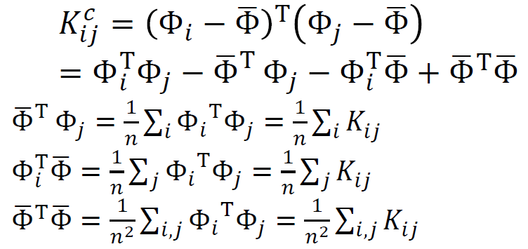
If we get the matrix K centered, then it is easy to calculate the alpha, the coefficient of z(the centered original data points). As you can see above, we can get centered K from just normal K and there is a more easy way to calculate the centered K because we know the centered K consists of normal K.

如果我们得到矩阵K居中，则很容易计算出alpha，即z的系数(居中的原始数据点)。正如您在上面看到的，我们可以仅从法线K获得中心K，并且有一种更简单的方法来计算中心K，因为我们知道中心K由法线K组成。

The proof to calculate the above equation is easy and we will skip this and the algorithm is the same with previous PCA because we know the centered K.

计算上面方程的证明很容易，我们将跳过这一点，并且算法与以前的PCA相同，因为我们知道中心K。

Algorithm

算法

Input: features and kernel function

输入：功能和内核功能

Output: Embedded value

输出：内含价值

Compute kernel matrix K.
计算内核矩阵K。
Compute centered K by HKH.
以HKH为中心计算K。
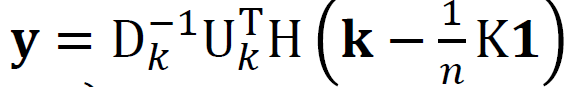
Compute spectral decomposition centered K = UΛU.transpose, sort the eigenvalue and eigenvectors in decreasing order of eigenvalues
计算以K =UΛU为中心的频谱分解。转置，按特征值的降序对特征值和特征向量进行排序
We select the desired dimension and D is the squared root of Λ only including desired dimensions.
我们选择所需的尺寸，D是仅包含所需尺寸的Λ的平方根。

You can compare this result and the result above. Actually, it is really similar to each other.

您可以将此结果与上面的结果进行比较。实际上，它们确实彼此相似。

Advantages

优点

Better reflects nonlinear structures.
更好地反映非线性结构。
Given suitable kernels, can be applied to more abstract objects or to unfold manifolds.
给定适当的内核，可以将其应用于更多抽象的对象或展开流形。

Disadvantages

缺点

Less interpretable because principal modes are no longer a fixed combination of input variables
难以解释，因为主体模式不再是输入变量的固定组合
Unlike with linear PCA, it is not easy to find a vector that corresponds to given Kernel PCA coordinates.
与线性PCA不同，要找到与给定内核PCA坐标相对应的向量并不容易。

Example

例

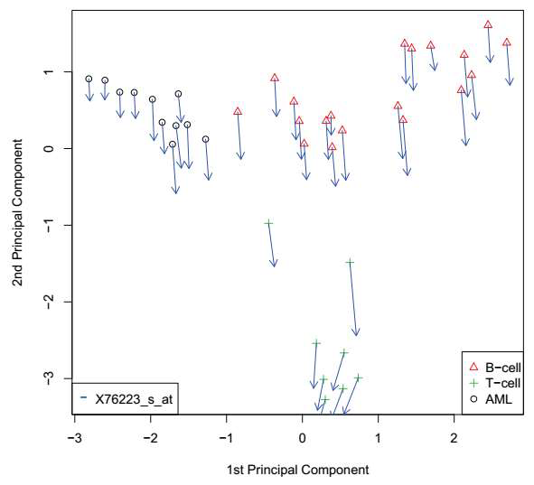
The graph is from Kernel PCA of gene expression data and the kernel is RBF kernel. The arrow indicates how much each point is changed when the single gene’s expression changes. As you can see, T-cell changes a lot but another cell dose not change much.

该图来自基因表达数据的内核PCA，内核为RBF内核。箭头指示当单个基因的表达改变时，每个点改变了多少。如您所见，T细胞变化很大，但另一个细胞变化不大。

This can be detected in other experiments. Therefore, Kernel PCA can represent its data well.

这可以在其他实验中检测到。因此，内核PCA可以很好地表示其数据。

The next post will be MDS and ISOMAP.

下一篇文章将是MDS和ISOMAP。

This post is published on 9/5/2020.This post is edited on 9/8/2020.

这篇文章发布于2020年9月5日这篇文章编辑于2020年9月8日

翻译自: https://medium.com/swlh/vc-high-dimensional-pca-and-kernel-pca-415ef47e2d15

pca vc

weixin_26632361

关注

0
点赞
踩
0

收藏

觉得还不错? 一键收藏
0
评论
pca vc_vc高维pca和内核pca

pca vcThis post assumes you already know what PCA is. If you don’t please check my previous post. 这篇文章假定您已经知道PCA是什么。如果您不这样做，请检查我以前的帖子。 n <p情况(高维PCA) (n < p case (High dimensional PCA))If th...
复制链接

扫一扫