


神经网络 代码python
机器学习 , 学术 , 教程 (Machine Learning, Scholarly, Tutorial)
Author(s): Pratik Shukla, Roberto Iriondo
作者:Pratik Shukla,Roberto Iriondo
Last updated, June 30, 2020
上次更新时间:2020年6月30日
In the first part of our tutorial on neural networks, we explained the basic concepts about neural networks, from the math behind them to implementing neural networks in Python without any hidden layers. We showed how to make satisfactory predictions even in case scenarios where we did not use any hidden layers. However, there are several limitations to single-layer neural networks.
在神经网络教程的第一部分中,我们解释了有关神经网络的基本概念,从其背后的数学到在Python中没有任何隐藏层的实现神经网络。 我们展示了即使在不使用任何隐藏层的情况下,如何做出令人满意的预测。 但是,单层神经网络存在一些限制。
In this tutorial, we will dive in-depth on the limitations and advantages of using neural networks in machine learning. We will show how to implement neural nets with hidden layers and how these lead to a higher accuracy rate on our predictions, along with implementation samples in Python on Google Colab.
在本教程中,我们将深入探讨在机器学习中使用神经网络的局限性和优势。 我们将展示如何使用隐藏层实现神经网络,以及如何在我们的预测中提高隐藏率,以及Google Colab中Python的实现示例。
指数: (Index:)
The general structure of an artificial neural network (ANN).
1.神经网络的局限性和优势 (1. Limitations and Advantages of Neural Networks)
单层神经网络的局限性: (Limitations of single-layer neural networks:)
- They can only represent a limited set of functions. If we have been training a model that uses complicated functions (which is the general case), then using a single layer neural network can lead to low accuracy in our prediction rate. 它们只能代表一组有限的功能。 如果我们一直在训练使用复杂函数的模型(这是一般情况),那么使用单层神经网络可能会导致我们的预测率准确性降低。
- They can only predict linearly separable data. If we have non-linear data, then training our single-layer neural network will lead to low accuracy in our prediction rate. 他们只能预测线性可分离的数据。 如果我们具有非线性数据,那么训练我们的单层神经网络将导致我们的预测率准确性降低。
- Decision boundaries for single-layer neural networks must be in the hyperplane, which means that if our data distributes in 3 dimensions, then our decision boundary must be in 2 dimensions. 单层神经网络的决策边界必须在超平面中,这意味着如果我们的数据以3维分布,则我们的决策边界必须以2维分布。

To overcome such limitations, we use hidden layers in our neural networks.
为了克服这些限制,我们在神经网络中使用了隐藏层。
单层神经网络的优点: (Advantages of single-layer neural networks:)
- Single-layer neural networks are easy to set up. 单层神经网络很容易建立。
- Single-layer neural networks take less time to train compared to a multi-layer neural network. 与多层神经网络相比,单层神经网络花费的时间更少。
- Single-layer neural networks have explicit links to statistical models. 单层神经网络与统计模型有明确的链接。
- The outputs in single layer neural networks are weighted sums of inputs. It means that we can interpret the output of a single layer neural network feasibly. 单层神经网络中的输出是输入的加权和。 这意味着我们可以切实地解释单层神经网络的输出。
多层神经网络的优点: (Advantages of multilayer neural networks:)
- They construct more extensive networks by considering layers of processing units. 他们通过考虑处理单元的层来构建更广泛的网络。
- They can be used to classify non-linearly separable data. 它们可用于对非线性可分离数据进行分类。
- Multilayer neural networks are more reliable compared to single-layer neural networks. 与单层神经网络相比,多层神经网络更可靠。
2.如何在隐藏层中选择几个神经元? (2. How to select several neurons in a hidden layer?)
There are many methods for determining the correct number of neurons to use in the hidden layer. We will see a few of them here.
有许多方法可以确定要在隐藏层中使用的神经元的正确数量。 我们将在这里看到其中的一些。
- The number of hidden nodes should be less than twice the size of the nodes in the input layer. 隐藏节点的数量应小于输入层中节点大小的两倍。
For example: If we have 2 input nodes, then our hidden nodes should be less than 4.
例如:如果我们有2个输入节点,那么我们的隐藏节点应小于4。
a. 2 inputs, 4 hidden nodes:
一个。 2个输入,4个隐藏节点:

b. 2 inputs, 3 hidden nodes:
b。 2个输入,3个隐藏节点:

c. 2 inputs, 2 hidden nodes:
C。 2个输入,2个隐藏节点:

d. 2 inputs, 1 hidden node:
d。 2个输入,1个隐藏节点:

- The number of hidden nodes should be 2/3 the size of input nodes, plus the size of the output node. 隐藏节点的数量应为输入节点大小的2/3加上输出节点的大小。
For example: If we have 2 input nodes and 1 output node then the hidden nodes should be = floor(2*2/3 + 1) = 2
例如:如果我们有2个输入节点和1个输出节点,则隐藏节点应为= floor(2 * 2/3 + 1)= 2
a. 2 inputs, 2 hidden nodes:
一个。 2个输入,2个隐藏节点:

- The number of hidden nodes should be between the size of input nodes and output nodes. 隐藏节点的数量应在输入节点和输出节点的大小之间。
For example: If we have 3 input nodes and 2 output nodes, then the hidden nodes should be between 2 and 3.
例如:如果我们有3个输入节点和2个输出节点,则隐藏节点应在2到3之间。
a. 3 inputs, 2 hidden nodes, 2 outputs:
一个。 3个输入,2个隐藏节点,2个输出:

b. 3 inputs, 3 hidden nodes, 2 outputs:
b。 3个输入,3个隐藏节点,2个输出:

我们需要多少个体重值? (How many weight values do we need?)
- For a hidden layer: Number of inputs * No. of hidden layer nodes 对于隐藏层:输入数量*隐藏层节点数
- For an output layer: Number of hidden layer nodes * No. of outputs 对于输出层:隐藏层节点数*输出数量
3.人工神经网络(ANN)的一般结构: (3. The General Structure of an Artificial Neural Network (ANN):)

人工神经网络的概述: (Summarization of an artificial neural network:)
- Take inputs. 接受输入。
- Add bias (if required). 添加偏见(如果需要)。
- Assign random weights in the hidden layer and the output layer. 在隐藏层和输出层中分配随机权重。
- Run the code for training. 运行代码进行培训。
- Find the error in prediction. 查找预测中的错误。
- Update the weight values of the hidden layer and output layer by gradient descent algorithm. 通过梯度下降算法更新隐藏层和输出层的权重值。
- Repeat the training phase with updated weights. 使用更新的权重重复训练阶段。
- Make predictions. 作出预测。
多层神经网络的执行: (Execution of multilayer neural networks:)
After reading the first article, we saw that we had only 1 phase of execution there. In that phase, we find the updated weight values and rerun the code to achieve minimum error. However, things are a little spicy here. The execution in a multilayer neural network takes place in two-phase. In phase-1, we update the values of weight_output (weight values for output layer), and in phase-2, we update the value of weight_hidden ( weight values for the hidden layer ). Phase-1 is similar to that of a neural network without any hidden layers.
阅读第一篇文章后,我们看到那里只有一个执行阶段。 在该阶段,我们找到更新的权重值,然后重新运行代码以实现最小错误。 但是,这里的东西有点辣。 多层神经网络中的执行分两阶段进行。 在阶段1中,我们更新weight_output的值(输出层的权重值),在阶段2中,我们更新weight_hidden的值(隐藏层的权重值)。 第一阶段类似于没有任何隐藏层的神经网络。
在第一阶段执行: (Execution in phase-1:)
To find the derivative, we are going to use in gradient descent algorithm to update the weight values. Here we are not going to derive the derivatives for those functions we already did in part -1 of neural network.In this phase, our goal is to find the weight values for the output layer. Here we are going to calculate the change in error concerning the change in output weight.
为了找到导数,我们将使用梯度下降算法来更新权重值。 在这里,我们将不为在神经网络的第-1部分中已经完成的那些函数导出导数。在此阶段,我们的目标是找到输出层的权重值。 在这里,我们将计算与输出重量变化有关的误差变化。
We first define some terms we are going to use in these derivatives:
我们首先定义将在这些派生词中使用的一些术语:

a. Finding the first derivative:
一个。 查找一阶导数:

b. Finding the second derivative:
b。 寻找二阶导数:
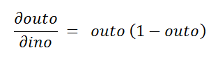
c. Finding the third derivative:
C。 找到三阶导数:

Notice that we already derived these derivatives in the first part of our tutorial.
在第二阶段执行: (Execution in phase-2:)
In phase-1, we find the updated weight for the output layer. In the second phase, we need to find the updated weights for the hidden layer. Hence, find how the change in hidden weight affects the change in error value.
在阶段1中,我们找到了输出层的更新权重。 在第二阶段,我们需要找到隐藏层的更新权重。 因此,发现隐藏权重的变化如何影响误差值的变化。
Represented as:
表示为:
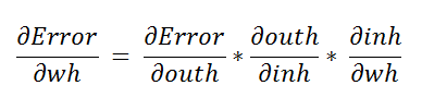
a. Finding the first derivative:
一个。 查找一阶导数:
Here we are going to use the chain rule to find the derivative.
在这里,我们将使用链式规则找到导数。
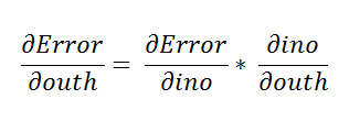
Using the chain rule again.
再次使用链式规则。
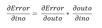
The step below is similar to what we did in the first part of our tutorial on neural networks.
下面的步骤类似于我们在神经网络教程的第一部分中所做的步骤。

b. Finding the second derivative:
b。 寻找二阶导数:

c. Finding the third derivative:
C。 找到三阶导数:

4.用Python实现多层神经网络 (4. Implementation of a multilayer neural network in Python)
📚 Multilayer neural network: A neural network with a hidden layer 📚 For more definitions, check out our article in terminology in machine learning.
Below we are going to implement the “OR” gate without the bias value. In conclusion, adding hidden layers in a neural network helps us achieve higher accuracy in our models.
下面我们将在没有偏置值的情况下实现“或”门。 总之,在神经网络中添加隐藏层有助于我们在模型中实现更高的准确性。
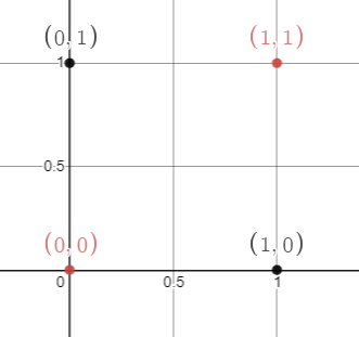
表示: (Representation:)

真值表: (Truth-Table:)

神经网络: (Neural Network:)
Notice that here we have 2 input features and 1 output feature. In this neural network, we are going to use 1 hidden layer with 3 nodes.
请注意,这里我们有2个输入功能和1个输出功能。 在这个神经网络中,我们将使用1个具有3个节点的隐藏层。

图示: (Graphical representation:)

用Python实现: (Implementation in Python:)
Below, we are going to implement our neural net with hidden layers step by step in Python, let’s code:
下面,我们将在Python中逐步实现带有隐藏层的神经网络,让我们编写代码:
a. Import required libraries:
一个。 导入所需的库:

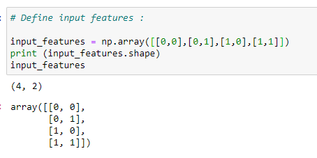
b. Define input features:
b。 定义输入功能:
Next, we take input values for which we want to train our neural network. We can see that we have taken two input features. On tangible data sets, the value of input features is mostly high.
接下来,我们输入要为其训练神经网络的输入值。 我们可以看到我们采用了两个输入功能。 在有形数据集上,输入要素的价值通常很高。

c. Define target output values:
C。 定义目标输出值:
For the input features, we want to have a specific output for specific input features. It is called the target output. We are going to train the model that gives us the target output for our input features.
对于输入要素,我们希望有针对特定输入要素的特定输出。 它称为目标输出。 我们将训练模型,该模型为我们的输入功能提供目标输出。

d. Assign random weights:
d。 分配随机权重:
Next, we are going to assign random weights to the input features. Note that our model is going to modify these weight values to be optimal. At this point, we are taking these values randomly. Here we have two layers, so we have to assign weights for them separately.
接下来,我们将为输入要素分配随机权重。 请注意,我们的模型将修改这些权重值以使其最佳。 此时,我们正在随机获取这些值。 在这里,我们有两层,因此我们必须分别为其分配权重。
The other variable is the learning rate. We are going to use the learning rate (LR) in a gradient descent algorithm to update the weight values. Generally, we keep LR as low as possible so that we can achieve a minimal error rate.
另一个变量是学习率。 我们将在梯度下降算法中使用学习率(LR)来更新权重值。 通常,我们将LR保持尽可能低,以使错误率最小。

e. Sigmoid function:
e。 乙状结肠功能:
Once we have our weight values and input features, we are going to send it to the main function that predicts the output. Notice that our input features and weight values can be anything, but here we want to classify data, so we need the output between 0 and 1. For such output, we are going to use a sigmoid function.
一旦我们有了权重值和输入特征,就将其发送给预测输出的主要功能。 注意,我们的输入特征和权重值可以是任何值,但是这里我们要对数据进行分类,因此我们需要0到1之间的输出。对于这种输出,我们将使用S型函数。

f. Sigmoid function derivative:
F。 乙状结肠功能导数:
In a gradient descent algorithm, we need the derivative of the sigmoid function.
在梯度下降算法中,我们需要S型函数的导数。

g. The main logic for predicting output and updating the weight values:
G。 预测输出并更新重量值的主要逻辑:
We are going to understand the following code step-by-step.
我们将逐步理解以下代码。


它是如何工作的? (How does it work?)
a. First of all, we run the above code 2,00,000 times. Keep in mind that if we only run this code a few times, then it is probable that we will have a higher error rate. Therefore, we update the weight values 10,000 times to reach the optimal value possible.
一个。 首先,我们将上面的代码运行2,00,000次。 请记住,如果我们只运行几次该代码,那么我们的错误率可能会更高。 因此,我们将权重值更新10,000次以达到可能的最佳值。
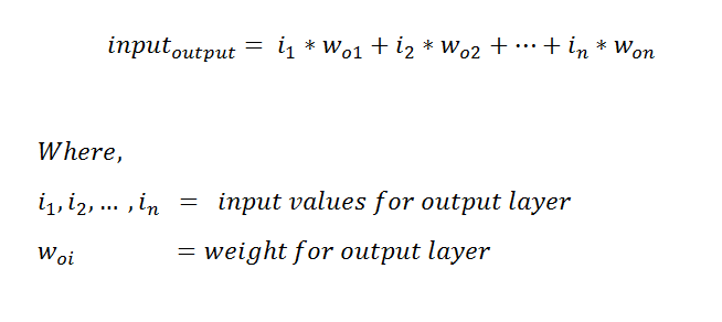
b. Next, we find the input for the hidden layer. Defined by the following formula:
b。 接下来,我们找到隐藏层的输入。 由以下公式定义:

We can also represent it as matrices to understand in a better way.
我们还可以将其表示为更好理解的矩阵。
The first matrix here is input features with size (4*2), and the second matrix is weight values for a hidden layer with size (2*3). So the resultant matrix will be of size (4*3).
这里的第一个矩阵是大小为(4 * 2)的输入要素,第二个矩阵是大小为(2 * 3)的隐藏层的权重值。 因此,所得矩阵的大小将为(4 * 3)。
The intuition behind the final matrix size:
最终矩阵大小的直觉是:
The row size of the final matrix is the same as the row size of the first matrix, and the column size of the final matrix is the same as the column size of the second matrix in multiplication (dot product).
最终矩阵的行大小与第一个矩阵的行大小相同,并且最终矩阵的列大小与第二个矩阵的列大小相乘(点积)。
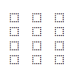
In the representation below, each of those boxes represents a value.
在下面的表示中,每个框代表一个值。

c. Afterward, we have an input for the hidden layer, and it is going to calculate the output by applying a sigmoid function. Below is the output of the hidden layer:
C。 之后,我们为隐藏层提供了一个输入,它将通过应用S形函数来计算输出。 以下是隐藏层的输出:

d. Next, we multiply the output of the hidden layer with the weight of the output layer:
d。 接下来,我们将隐藏层的输出乘以输出层的权重:
The first matrix shows the output of the hidden layer, which has a size of (4*3). The second matrix represents the weight values of the output layer,
第一个矩阵显示隐藏层的输出,其大小为(4 * 3)。 第二个矩阵代表输出层的权重值,

e. Afterward, we calculate the output of the output layer by applying a sigmoid function. It can also be represented in matrix form as follows.
e。 然后,我们通过应用S形函数来计算输出层的输出。 它也可以如下矩阵形式表示。

f. Now that we have our predicted output, we find the mean squared between target output and predicted output.
F。 现在我们有了预测的输出,我们找到了目标输出和预测的输出之间的均方。

g. Next, we begin the first phase of training. In this step, we update the weight values for the output layer. We need to find out how much the output weights affect the error value. To update the weights, we use a gradient descent algorithm. Notice that we have already found the derivatives we will use during the training phase.
G。 接下来,我们开始训练的第一阶段。 在此步骤中,我们将更新输出图层的权重值。 我们需要找出输出权重对误差值有多大影响。 要更新权重,我们使用梯度下降算法。 请注意,我们已经找到了在训练阶段将使用的派生工具。

g.a. Matrix representation of the first derivative. Matrix size (4*1).
ga一阶导数的矩阵表示形式。 矩阵大小(4 * 1)。
derror_douto = output_op -target_output
derror_douto = output_op -target_output

g.b. Matrix representation of the second derivative. Matrix size (4*1).
gb二阶导数的矩阵表示形式。 矩阵大小(4 * 1)。
dout_dino = sigmoid_der(input_op)
dout_dino = sigmoid_der(input_op)

g.c. Matrix representation of the third derivative. Matrix size (4*3).
gc三阶导数的矩阵表示。 矩阵大小(4 * 3)。
dino_dwo = output_hidden
dino_dwo = output_hidden

g.d. Matrix representation of transpose of dino_dwo. Matrix size (3*4).
gd dino_dwo转置的矩阵表示dino_dwo 。 矩阵大小(3 * 4)。

g.e. Now, we are going to find the final matrix of output weight. For a detailed explanation of this step, please check out our previous tutorial. The matrix size will be (3*1), which is the same as the output_weight matrix.
现在,GE,我们会发现输出权的最终矩阵。 有关此步骤的详细说明,请查看我们以前的教程 。 矩阵大小将为(3 * 1),与output_weight矩阵相同。

Hence, we have successfully find the derivative values. Next, we update the weight values accordingly with the help of a gradient descent algorithm.
因此,我们已经成功找到了导数值。 接下来,我们借助梯度下降算法相应地更新权重值。
Nonetheless, we also have to find the derivative for phase-2. Let’s first find that, and then we will update the weights for both layers in the end.
尽管如此,我们还必须找到第二阶段的导数。 首先找到它,然后最后更新两个图层的权重。
h. Phase -2. Updating the weights in the hidden layer.
H。 阶段2。 更新隐藏层中的权重。
Since we have already discussed how we derived the derivative values, we are just going to see matrix representation for each of them to understand it better. Our goal here is to find the weight matrix for the hidden layer, which is of size (2*3).
由于我们已经讨论了如何导出微分值,因此我们将看到它们每个的矩阵表示形式,以便更好地理解它。 我们的目标是找到隐藏层的权重矩阵,其大小为(2 * 3)。
h.a. Matrix representation for the first derivative.
ha一阶导数的矩阵表示形式。
derror_dino = derror_douto * douto_dino
derror_dino = derror_douto * douto_dino

h.b. Matrix representation for the second derivative.
hb二阶导数的矩阵表示。
dino_douth = weight_output
dino_douth = weight_output

h.c. Matrix representation for the third derivative.
hc三阶导数的矩阵表示形式。
derror_douth = np.dot(derror_dino , dino_douth.T)
derror_douth = np.dot(derror_dino , dino_douth.T)

h.d. Matrix representation for the fourth derivative.
hd四阶导数的矩阵表示形式。
douth_dinh = sigmoid_der(input_hidden)
douth_dinh = sigmoid_der(input_hidden)
h.e. Matrix representation for the fifth derivative.
他矩阵表示为第五衍生物。
dinh_dwh = input_features
dinh_dwh = input_features

h.f. Matrix representation for the sixth derivative.
hf六阶导数的矩阵表示形式。
derror_dwh = np.dot(dinh_dwh.T, douth_dinh * derror_douth)
derror_dwh = np.dot(dinh_dwh.T, douth_dinh * derror_douth)

Notice that our goal was to find a hidden weight matrix with the size of (2*3). Furthermore, we have successfully managed to find it.
注意,我们的目标是找到一个大小为(2 * 3)的隐藏权重矩阵。 此外,我们已经成功地找到了它。
h.g. Updating the weight values :
hg更新重量值:
We will use the gradient descent algorithm to update the values. It takes three parameters.
我们将使用梯度下降算法来更新值。 它包含三个参数。
- The original weight: we already have it. 原始重量:我们已经拥有了。
- The learning rate (LR): we assigned it the value of 0.05. 学习率(LR):我们将其指定为0.05。
- The derivative: Found on the previous step. 导数:在上一步中找到。
Gradient descent algorithm:
梯度下降算法:

Since we have all of our parameter values, this will be a straightforward operation. First, we are updating the weight values for the output layer, and then we are updating the weight values for the hidden layer.
由于我们拥有所有参数值,因此这将是一个简单的操作。 首先,我们更新输出层的权重值,然后更新隐藏层的权重值。
i. Final weight values:
一世。 最终重量值:
Below, we show the updated weight values for both layers — our prediction bases on these values.
下面,我们显示了两层的更新权重值-我们基于这些值的预测。


j. Making predictions:
j。 做出预测:
j.a. Prediction for (1,1).
ja (1,1)的预测。
Target output = 1
目标输出= 1
Explanation:
说明:
First of all, we are going to take the input values for which we want to predict the output. The “result1” variable stores the value of the dot product of input variables and hidden layer weight. We obtain the output by applying a sigmoid function, the result stores in the result2 variable. Such is the input feature for the output layer. We calculate the input for the output layer by multiplying input features with output layer weight. To find the final output value, we take the sigmoid value of that.
首先,我们将采用要为其预测输出的输入值。 “ result1”变量存储输入变量和隐藏层权重的点积值。 我们通过应用S型函数来获得输出,结果存储在result2变量中。 这就是输出层的输入功能。 我们通过将输入要素乘以输出层权重来计算输出层的输入。 为了找到最终的输出值,我们采用其S形值。

Notice that the predicted output is very close to 1. So we have managed to make accurate predictions.
请注意,预测的输出非常接近1。因此,我们已经做出了准确的预测。
j.b. Prediction for (0,0).
jb (0,0)的预测。
Target output = 0
目标输出= 0

Note that the predicted output is very close to 0, which indicates the success rate of our model.
请注意,预测输出非常接近0,这表明我们模型的成功率。
k. Final error value :
k。 最终错误值:
After 200,000 iterations, we have our final error value — the lower the error, the higher the accuracy of the model.
经过20万次迭代后,我们得到了最终的误差值-误差越小,模型的精度越高。

As shown above, we can see that the error value is 0.0000000189. This value is the final error value in prediction after 200,000 iterations.
如上所示,我们可以看到错误值为0.0000000189。 该值是200,000次迭代后预测中的最终误差值。
放在一起: (Putting it all together:)
# Import required libraries :
import numpy as np# Define input features :
input_features = np.array([[0,0],[0,1],[1,0],[1,1]])
print (input_features.shape)
print (input_features)# Define target output :
target_output = np.array([[0,1,1,1]])# Reshaping our target output into vector :
target_output = target_output.reshape(4,1)
print(target_output.shape)
print (target_output)# Define weights :
# 6 for hidden layer
# 3 for output layer
# 9 totalweight_hidden = np.array([[0.1,0.2,0.3],
 [0.4,0.5,0.6]])
weight_output = np.array([[0.7],[0.8],[0.9]])# Learning Rate :
lr = 0.05# Sigmoid function :
def sigmoid(x):
 return 1/(1+np.exp(-x))# Derivative of sigmoid function :
def sigmoid_der(x):
 return sigmoid(x)*(1-sigmoid(x))for epoch in range(200000):
 # Input for hidden layer :
 input_hidden = np.dot(input_features, weight_hidden)

 # Output from hidden layer :
 output_hidden = sigmoid(input_hidden)

 # Input for output layer :
 input_op = np.dot(output_hidden, weight_output)

 # Output from output layer :
 output_op = sigmoid(input_op)#==========================================================
 # Phase1

 # Calculating Mean Squared Error :
 error_out = ((1 / 2) * (np.power((output_op — target_output), 2)))
 print(error_out.sum())

 # Derivatives for phase 1 :
 derror_douto = output_op — target_output
 douto_dino = sigmoid_der(input_op)
 dino_dwo = output_hiddenderror_dwo = np.dot(dino_dwo.T, derror_douto * douto_dino)#===========================================================
 # Phase 2
 # derror_w1 = derror_douth * douth_dinh * dinh_dw1
 # derror_douth = derror_dino * dino_outh

 # Derivatives for phase 2 :
 derror_dino = derror_douto * douto_dino
 dino_douth = weight_output
 derror_douth = np.dot(derror_dino , dino_douth.T)
 douth_dinh = sigmoid_der(input_hidden)
 dinh_dwh = input_features
 derror_wh = np.dot(dinh_dwh.T, douth_dinh * derror_douth)# Update Weights
 weight_hidden -= lr * derror_wh
 weight_output -= lr * derror_dwo

# Final hidden layer weight values :
print (weight_hidden)# Final output layer weight values :
print (weight_output)# Predictions :#Taking inputs :
single_point = np.array([1,1])
#1st step :
result1 = np.dot(single_point, weight_hidden)
#2nd step :
result2 = sigmoid(result1)
#3rd step :
result3 = np.dot(result2,weight_output)
#4th step :
result4 = sigmoid(result3)
print(result4)#=================================================
#Taking inputs :
single_point = np.array([0,0])
#1st step :
result1 = np.dot(single_point, weight_hidden)
#2nd step :
result2 = sigmoid(result1)
#3rd step :
result3 = np.dot(result2,weight_output)
#4th step :
result4 = sigmoid(result3)
print(result4)#=====================================================
#Taking inputs :
single_point = np.array([1,0])
#1st step :
result1 = np.dot(single_point, weight_hidden)
#2nd step :
result2 = sigmoid(result1)
#3rd step :
result3 = np.dot(result2,weight_output)
#4th step :
result4 = sigmoid(result3)
print(result4)
Below, notice that the data we used in this example was linearly separable, which means that by a single line, we can classify outputs with 1 value and outputs with 0 values.
在下面,请注意我们在本示例中使用的数据是线性可分离的,这意味着通过一行,我们可以将输出分为1个值和输出为0个值。

Launch it on Google Colab:
在Google Colab上启动它:
5.与单层神经网络的比较 (5. Comparison with a single-layer neural network)
Notice that we did not use bias value here. Now let’s have a quick look at the neural network without hidden layers for the same input features and target values. What we are going to do is find the final error rate and compare it. Since we have already implemented the code in our previous tutorial, for this purpose, we are going to analyze it quickly. [2]
注意,这里我们没有使用偏差值。 现在,让我们快速浏览一下具有相同输入特征和目标值的无隐藏层的神经网络。 我们要做的是找到最终的错误率并进行比较。 由于我们已经在上一教程中实现了该代码,因此,我们将对其进行快速分析。 [ 2 ]
The final error value for the following code is:
以下代码的最终错误值为:

As we can see, the error value is way too high compared to the error we found in our neural network implementation with hidden layers, making it one of the main reasons to use hidden layers in a neural network.
如我们所见,与在带有隐藏层的神经网络实现中发现的错误相比,该错误值太大了,这使其成为在神经网络中使用隐藏层的主要原因之一。
# Import required libraries :
import numpy as np# Define input features :
input_features = np.array([[0,0],[0,1],[1,0],[1,1]])
print (input_features.shape)
print (input_features)# Define target output :
target_output = np.array([[0,1,1,1]])# Reshaping our target output into vector :
target_output = target_output.reshape(4,1)
print(target_output.shape)
print (target_output)# Define weights :
weights = np.array([[0.1],[0.2]])
print(weights.shape)
print (weights)# Define learning rate :
lr = 0.05# Sigmoid function :
def sigmoid(x):
    return 1/(1+np.exp(-x))# Derivative of sigmoid function :
def sigmoid_der(x):
    return sigmoid(x)*(1-sigmoid(x))# Main logic for neural network :
# Running our code 10000 times :for epoch in range(10000):
    inputs = input_features#Feedforward input :
    pred_in = np.dot(inputs, weights)#Feedforward output :
    pred_out = sigmoid(pred_in)#Backpropogation
    #Calculating error
    error = pred_out - target_output
    x = error.sum()

    #Going with the formula :
    print(x)

    #Calculating derivative :
    dcost_dpred = error
    dpred_dz = sigmoid_der(pred_out)

    #Multiplying individual derivatives :
    z_delta = dcost_dpred * dpred_dz#Multiplying with the 3rd individual derivative :
    inputs = input_features.T
    weights -= lr * np.dot(inputs, z_delta)#Predictions :#Taking inputs :
single_point = np.array([1,0])
#1st step :
result1 = np.dot(single_point, weights)
#2nd step :
result2 = sigmoid(result1)
#Print final result
print(result2)#====================================
#Taking inputs :
single_point = np.array([0,0])
#1st step :
result1 = np.dot(single_point, weights)
#2nd step :
result2 = sigmoid(result1)
#Print final result
print(result2)#===================================
#Taking inputs :
single_point = np.array([1,1])
#1st step :
result1 = np.dot(single_point, weights)
#2nd step :
result2 = sigmoid(result1)
#Print final result
print(result2)
Launch it on Google Colab:
在Google Colab上启动它:
6.带有神经网络的非线性可分离数据 (6. Non-linearly separable data with a neural network)
In this example, we are going to take a dataset that cannot be separated by a single straight line. If we try to separate it by a single line, then one or many outputs may be misclassified, and we will have a very high error. Therefore we use a hidden layer to resolve this issue.
在此示例中,我们将获取无法用一条直线分开的数据集。 如果我们试图用一行将其分开,那么一个或多个输出可能会被错误分类,并且我们将有很高的误差。 因此,我们使用隐藏层来解决此问题。
输入表: (Input Table:)

数据点的图形表示: (Graphical Representation Of Data Points :)
As shown below, we represent the data on the coordinate plane. Here notice that we have 2 colored dots (black and red). If we try to draw a single line, then the output is going to be misclassified.
如下所示,我们在坐标平面上表示数据。 在这里请注意,我们有2个彩色的点(黑色和红色)。 如果我们试图画一条线,那么输出将被错误分类。
As figure 59 shows, we have 2 inputs and 1 output. In this example, we are going to use 4 hidden perceptrons. The red dots have an output value of 0, and the black dots have an output value of 1. Therefore, we cannot simply classify them using a single straight line.
如图59所示,我们有2个输入和1个输出。 在此示例中,我们将使用4个隐藏的感知器。 红点的输出值为0,黑点的输出值为1。因此,我们不能简单地使用一条直线对它们进行分类。
神经网络: (Neural Network:)

用Python实现: (Implementation in Python:)
a. Import required libraries:
一个。 导入所需的库:

b. Define input features:
b。 定义输入功能:
c. Define the target output:
C。 定义目标输出:

d. Assign random weight values:
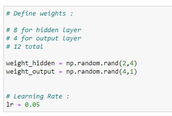
d。 分配随机权重值:
On figure 64, notice that we are using NumPy’s library random function to generate random values.
在图64上,请注意,我们正在使用NumPy的库随机函数来生成随机值。
numpy.random.rand(x,y): Here x is the number of rows, and y is the number of columns. It generates output values over [0,1). It means 0 is included, but 1 is not included in the value generation.
numpy.random.rand(x,y) :这里x是行数,y是列数。 它生成超过[0,1)的输出值。 这意味着在值生成中包括了0,但没有包括1。
e. Sigmoid function:
e。 乙状结肠功能:

f. Finding the derivative with a sigmoid function:
F。 用S型函数查找导数:

g. Training our neural network:
G。 训练我们的神经网络:


h. Weight values of hidden layer:
H。 隐藏层的权重值:

i. Weight values of output layer:
一世。 输出层的权重值:

j. Final error value :
j。 最终错误值:
After training our model for 200,000 iterations, we finally achieved a low error value.
在对模型进行了200,000次迭代训练之后,我们最终实现了较低的误差值。

k. Making predictions from the trained model :
k。 根据训练后的模型做出预测:
k.a. Predicting output for (0.5, 2).
ka预测(0.5,2)的输出。

The predicted output is closer to 1.
预测输出接近于1。
k.b. Predicting output for (0, -1)
kb预测(0,-1)的输出
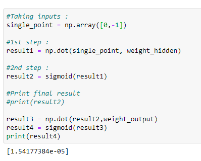
The predicted output is very near to 0.
预测的输出非常接近0。
k.c. Predicting output for (0, 5)
kc预测( 0,5)的输出

The predicted output is close to 1.
预测输出接近1。
k.d. Predicting output for (1, 1.2)
kd预测( 1,1.2)的输出

The predicted output is close to 0.
预测的输出接近于0。
Based on the output values, our model has done a high-grade job of predicting values.
基于输出值,我们的模型在预测值方面做得很好。
We can separate our data in the following way as shown in Figure 76. Note that this is not the only possible way to separate these values.
我们可以按照以下方式分离数据,如图76所示。请注意,这不是分离这些值的唯一可能方法。

Therefore to conclude, using a hidden layer on our neural networks helps us reducing the error rate when we have non-linearly separable data. Even though the training time extends, we have to remember that our goal is to make high accuracy predictions, and such will be satisfied.
因此,可以得出结论,在我们拥有非线性可分离数据时,在神经网络上使用隐藏层有助于降低错误率。 即使训练时间延长了,我们也必须记住我们的目标是做出高精度的预测,而这将得到满足。
放在一起: (Putting it all together:)
# Import required libraries :
import numpy as np# Define input features :
input_features = np.array([[0,0],[0,1],[1,0],[1,1]])
print (input_features.shape)
print (input_features)# Define target output :
target_output = np.array([[0,1,1,0]])# Reshaping our target output into vector :
target_output = target_output.reshape(4,1)
print(target_output.shape)
print (target_output)# Define weights :
# 8 for hidden layer
# 4 for output layer
# 12 total
weight_hidden = np.random.rand(2,4)
weight_output = np.random.rand(4,1)# Learning Rate :
lr = 0.05# Sigmoid function :
def sigmoid(x):
 return 1/(1+np.exp(-x))# Derivative of sigmoid function :
def sigmoid_der(x):
 return sigmoid(x)*(1-sigmoid(x))# Main logic :
for epoch in range(200000):
 # Input for hidden layer :
 input_hidden = np.dot(input_features, weight_hidden)

 # Output from hidden layer :
 output_hidden = sigmoid(input_hidden)

 # Input for output layer :
 input_op = np.dot(output_hidden, weight_output)

 # Output from output layer :
 output_op = sigmoid(input_op)#========================================================================
 # Phase1

 # Calculating Mean Squared Error :
 error_out = ((1 / 2) * (np.power((output_op — target_output), 2)))
 print(error_out.sum())


 # Derivatives for phase 1 :
 derror_douto = output_op — target_output
 douto_dino = sigmoid_der(input_op)
 dino_dwo = output_hiddenderror_dwo = np.dot(dino_dwo.T, derror_douto * douto_dino)# ========================================================================
 # Phase 2# derror_w1 = derror_douth * douth_dinh * dinh_dw1
 # derror_douth = derror_dino * dino_outh

 # Derivatives for phase 2 :
 derror_dino = derror_douto * douto_dino
 dino_douth = weight_output
 derror_douth = np.dot(derror_dino , dino_douth.T)
 douth_dinh = sigmoid_der(input_hidden)
 dinh_dwh = input_features
 derror_dwh = np.dot(dinh_dwh.T, douth_dinh * derror_douth)# Update Weights
 weight_hidden -= lr * derror_dwh
 weight_output -= lr * derror_dwo


# Final values of weight in hidden layer :
print (weight_hidden)# Final values of weight in output layer :
print (weight_output)#Taking inputs :
single_point = np.array([0,-1])
#1st step :
result1 = np.dot(single_point, weight_hidden)
#2nd step :
result2 = sigmoid(result1)
#3rd step :
result3 = np.dot(result2,weight_output)
#4th step :
result4 = sigmoid(result3)
print(result4)#Taking inputs :
single_point = np.array([0,5])
#1st step :
result1 = np.dot(single_point, weight_hidden)
#2nd step :
result2 = sigmoid(result1)
#3rd step :
result3 = np.dot(result2,weight_output)
#4th step :
result4 = sigmoid(result3)
print(result4)#Taking inputs :
single_point = np.array([1,1.2])
#1st step :
result1 = np.dot(single_point, weight_hidden)
#2nd step :
result2 = sigmoid(result1)
#3rd step :
result3 = np.dot(result2,weight_output)
#4th step :
result4 = sigmoid(result3)
print(result4)
Launch it on Google Colab:
在Google Colab上启动它:
7.结论 (7. Conclusion)
- Neural networks can learn from their mistakes, and they can produce output that is not limited to the inputs provided to them. 神经网络可以从错误中吸取教训,并且可以产生不仅限于提供给他们的输入的输出。
- Inputs store in its networks instead of a database. 输入存储在其网络中而不是数据库中。
- These networks can learn from examples, and we can predict the output for similar events. 这些网络可以从示例中学习,我们可以预测类似事件的输出。
- In case of failure of one neuron, the network can detect the fault and still produce output. 万一一个神经元发生故障,网络可以检测到故障并仍然产生输出。
- Neural networks can perform multiple tasks in parallel processes. 神经网络可以在并行过程中执行多个任务。
DISCLAIMER: The views expressed in this article are those of the author(s) and do not represent the views of Carnegie Mellon University, nor other companies (directly or indirectly) associated with the author(s). These writings do not intend to be final products, yet rather a reflection of current thinking, along with being a catalyst for discussion and improvement.
免责声明:本文中表达的观点仅为作者的观点,并不代表卡耐基梅隆大学或与作者相关的其他公司(直接或间接)的观点。 这些著作并非最终产品,而是当前思想的反映,同时也是讨论和改进的催化剂。
Published via Towards AI
通过Towards AI发布
推荐文章 (Recommended Articles)
I. Best Datasets for Machine Learning and Data ScienceII. AI Salaries Heading SkywardIII. What is Machine Learning?IV. Best Masters Programs in Machine Learning (ML) for 2020V. Best Ph.D. Programs in Machine Learning (ML) for 2020VI. Best Machine Learning BlogsVII. Key Machine Learning DefinitionsVIII. Breaking Captcha with Machine Learning in 0.05 SecondsIX. Machine Learning vs. AI and their Important DifferencesX. Ensuring Success Starting a Career in Machine Learning (ML)XI. Machine Learning Algorithms for BeginnersXII. Neural Networks from Scratch with Python Code and Math in DetailXIII. Building Neural Networks with Python
I. 机器学习和数据科学的最佳数据集 II。 AI薪水朝着Skyward III 前进 。 什么是机器学习? IV。 2020年 最佳 机器学习(ML)硕士课程 。 2020年机器学习(ML)程序 。 最佳机器学习博客 VII。 关键机器学习定义 VIII。 在0.05秒内用机器学习打破验证码 IX。 机器学习与AI及其重要区别 X. 确保成功开始机器学习(ML)的职业生涯 XI。 初学者 XII的机器学习算法 。 Scratch的神经网络,详细介绍了Python代码和数学 XIII。 使用Python构建神经网络
引文 (Citation)
For attribution in academic contexts, please cite this work as:
对于学术背景中的归因,请引用此作品为:
Shukla, et al., “Building Neural Networks with Python Code and Math in Detail — II”, Towards AI, 2020BibTex引文: (BibTex citation:)
@article{pratik_iriondo_2020,
 title={Building Neural Networks with Python Code and Math in Detail — II},
 url={https://towardsai.net/building-neural-nets-with-python},
 journal={Towards AI},
 publisher={Towards AI Co.},
 author={Pratik, Shukla and Iriondo, Roberto},
 year={2020},
 month={Jun}
}
📚 Are you new to machine learning? Check out an overview of machine learning algorithms for beginners with code examples in Python 📚
神经网络 代码python


 1358
1358

 被折叠的 条评论
为什么被折叠?
被折叠的 条评论
为什么被折叠?
 到【灌水乐园】发言


