批量归一化与量化推理模型的不同角度

Abstract :The Batch Normalization benefits in training are well known with reduction of internal covariate shift and hence optimizing the training to converge faster. This article tries to bring different perspective, where quantization loss is recovered with the help of Batch Normalization layer and hence retaining the accuracy of the model. The article also gives simplified implementation of Batch Normalization to reduce the load on edge devices which generally will have constraints on computation of neural network models.

摘要：通过减少内部协变量偏移并因此优化训练以使其收敛更快，训练中的“批量归一化”好处是众所周知的。 本文尝试提出不同的观点，即借助批归一化层可以恢复量化损失，从而保持模型的准确性。 本文还给出了批标准化的简化实现，以减少边缘设备的负载，这通常会对神经网络模型的计算产生限制。

批量归一化理论： (Batch Normalization Theory:)

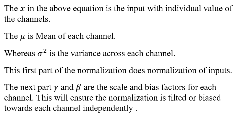
During training of neural network, we have to ensure that the network learns faster. One of the way to make it faster is by normalizing the inputs to network, along with normalization of intermittent layers of the network. This intermediate layer normalization is what is called Batch Normalization.The Advantage of Batch norm is also that it helps in minimizing internal covariate shift, as described in this paper .

在训练神经网络时，我们必须确保网络学习速度更快。 使其更快的一种方法是对网络的输入进行标准化，并对网络的间歇层进行标准化。 这种中间层归一化称为批处理归一化。批处理范数的优点还在于它有助于最小化内部协变量偏移，如本文所述 。

The frameworks like tensorflow,keras and caffe have got same representation with different symbols attached to it. In general the Batch Normalization can be described by following math:

tensorflow，keras和caffe之类的框架具有相同的表示形式，并带有不同的符号。 通常，可以通过以下数学描述批标准化：

Here the equation (1.1), is representation of keras/tensorflow. whereas equation (1.2) is representation used by caffe framework. In this article the equation (1.1) style is adopted for continuation of the context.

这里的等式(1.1)是角膜/张量流的表示。 而公式(1.2)是caffe框架使用的表示形式。 在本文中，采用等式(1.1)样式来延续上下文。

Now lets modify the equation (1.1) as below :

现在让我们修改等式(1.1)如下：

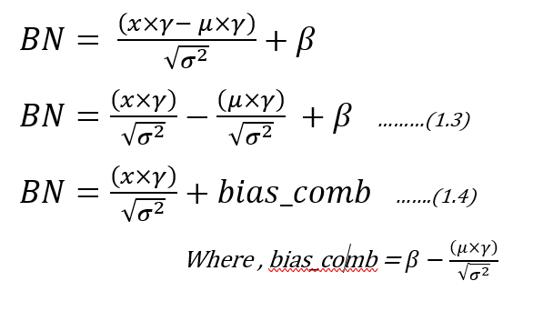
Now by observing equation of (1.4), there is option for optimization in reducing number of multiplications and additions. The bias_comb (read it as combined bias) factor can be offline calculated for each channel . Also the ratio of “gamma/sqrt(variance)”can be calculated offline and can be used while implementing the Batch norm equation. This equation can be used in Quantized inference model, to reduce the complexity.

现在，通过观察公式(1.4)，可以选择减少乘法和加法的数量的优化方法。 可以离线为每个通道计算bias_comb(作为组合偏差)因子。 同样，“伽玛/平方根(方差)”之比也可以离线计算，并且可以在执行Batch norm方程时使用。 该方程可用于量化推理模型，以降低复杂度。

量化推理模型 (Quantized Inference Model)

The inference model to be deployed in edge devices, would generally integer arithmetic friendly CPUs, such as ARM Cortex-M/A series processors or FPGA devices. Now to make inference model friendly to the architecture of the edge devices, will create a simulation in python. And then convert the inference model’s chain of inputs,weights and outputs in to fixed point format. The fixed point format,Q for 8 bits is chosen to represent with integer.fractional format. This simulation model will help you to develop inference model faster on device and also will help you to evaluate the accuracy of the model.

要在边缘设备中部署的推理模型通常将使用整数算法友好型CPU，例如ARM Cortex-M / A系列处理器或FPGA设备。 现在，为了使推理模型对边缘设备的体系结构友好，将在python中创建一个仿真。 然后将推理模型的输入，权重和输出链转换为定点格式。 选择8位的定点格式Q以整数。小数格式表示。 该仿真模型将帮助您在设备上更快地开发推理模型，还将帮助您评估模型的准确性。

e.g : Q2.6 represents 6 bits of fractional and 2 bits of integer.

例如：Q2.6代表6位小数和2位整数。

Now the way to represent the Q format for each layer is as follows:

现在，表示每层Q格式的方法如下：

1. Take the Maximum and Minimum of inputs,outputs and each layer/weights .
   取输入，输出和每个图层/权重的最大值和最小值。
2. Get the fractional bits required to represent the Dynamic range (by using Maximum/Minimum) is as below using python function:
   使用python函数获取代表动态范围所需的小数位(通过使用最大值/最小值)如下：

def get_fract_bits(tensor_float):
       # Assumption is that out of 8 bits, one bit is used as sign
       fract_dout = 7 - np.ceil(np.log2(abs(tensor_float).max()))       fract_dout = fract_dout.astype('int8')       return fract_dout

3. Now the integer bits are 7-fractional_bits, as one bit is reserved for sign representation.4. To start with perform this on input and then followed by Layer 1, 2 …, so on .5. Do the quantization step for weights and then for the output assuming one example of input. The assumption is made that input is normalized so that we can generalize the Q format, otherwise this may lead to some loss in data when non-normalized different input gets fed.6. This will set Q format for input,weights and outputs.

3.现在整数位是7-fractional_bits，因为保留一位用于符号表示。4。 首先在输入上执行此操作，然后执行第1层，第2层…，依此类推。.5。 假设输入的一个示例，对权重然后对输出进行量化步骤。 假设输入是标准化的，这样我们就可以推广Q格式，否则当输入非标准化的不同输入时，这可能会导致数据丢失。6。 这将为输入，权重和输出设置Q格式。

Example: Lets consider Resnet-50 as model to be quantized. Lets use Keras inbuilt Resnet-50 trained with Imagenet.

示例：让我们将Resnet-50视为要量化的模型。 让我们使用通过Imagenet培训的Keras内置Resnet-50。

#Creating the model 
def model_create():      model = tf.compat.v1.keras.applications.resnet50.ResNet50(include_top=True, weights='imagenet', input_tensor=None, input_shape=None,pooling=None, classes=1000)      return model

Lets prepare an input for resnet-50. The below image is taken from Imgenet dataset.

让我们为resnet-50准备输入。 下图取自Imgenet数据集。

Elephant Image from Imgenet data.

来自Imgenet数据的大象图像。

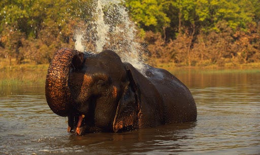
def prepare_input():       img = image.load_img("D:\\Elephant_water.jpg",target_size=(224,224))       x_test = image.img_to_array(img)       x_test = np.expand_dims(x_test,axis=0)       x = preprocess_input(x_test) # from tensorflow.compat.v1.keras.applications.resnet50 import preprocess_input, decode_predictions       return x

Now Lets call the above two functions and find out the Q format for input.

现在，让我们调用上述两个函数并找出Q格式进行输入。

model = model_create()x = prepare_input()

If you observe the input ‘x’, its dynamic range is between -123.68 to 131.32. This makes it hard for fitting in 8 bits, as we only have 7 bits to represent these numbers, considering one sign bit. Hence the Q Format for this input would become, Q8.0, where 7 bits are input numbers and 1 sign bit. Hence it clips the data between -128 to +127 (-2⁷ to 2⁷ -1). so we would be loosing some data in this input quantization conversion (most obvious being 131.32 is clipped to 127), whose loss can be seen by Signal to Quantize Noise Ratio , which will be described soon below.

如果观察到输入“ x”，则其动态范围在-123.68至131.32之间。 考虑到一个符号位，这使它很难适合8位，因为我们只有7位代表这些数字。 因此，此输入的Q格式将变为Q8.0，其中7位是输入数字和1个符号位。 因此，它将数据剪辑在-128至+127(-2⁷至2⁷-1)之间。 因此，我们将在此输入量化转换中丢失一些数据(最明显的是131.32被限制为127)，其损失可以通过信噪比(见下文)进行说明。

If you follow the same method for each weight and outputs of the layers, we will have some Q format which we can fix to simulate the quantization.

如果您对图层的每个权重和输出采用相同的方法，我们将获得一些Q格式，可以修复该格式以模拟量化。

# Lets get first layer properties(padding, _) = model.layers[1].padding# lets get second layer propertieswts = model.layers[2].get_weights()strides = model.layers[2].stridesW=wts[0]b=wts[1]hparameters =dict(pad=padding[0],stride=strides[0])# Lets Quantize the weights .quant_bits = 8 # This will be our data path.wts_qn,wts_bits_fract = Quantize(W,quant_bits) # Both weights and biases will be quantized with wts_bits_fract.# lets quantize Bias also at wts_bits_fractb_qn = (np.round(b *(2<<wts_bits_fract))).astype('int8')names_model,names_pair = getnames_layers(model)layers_op = get_each_layers(model,x,names_model)quant_bits = 8print("Running conv2D")# Lets extract the first layer output from convolution block.Z_fl = layers_op[2] # This Number is first convolution.# Find out the maximum bits required for final convolved value.fract_dout = get_fract_bits(Z_fl)fractional_bits = [0,wts_bits_fract,fract_dout]# Quantized convolution here.
Z, cache_conv = conv_forward(x.astype('int8'),wts_qn, b_qn[np.newaxis,np.newaxis,np.newaxis,...], hparameters,fractional_bits)

Now if you observe the above snippet of code, the convolution operation will take input , weights and output with its fractional bits defined.i.e: fractional_bits=[0,7,-3]where 1st element represents 0 bits for fractional representation of input (Q8.0)2nd element represents 7 bits for fractional representation of weights (Q1.7).3rd element represents -3 bits for fractional representation of outputs (Q8.0, but need additional 3 bits for integer representation as range is beyond 8 bit representation).

现在，如果您观察上面的代码片段，则卷积操作将使用input，weights和output及其定义的小数位。即：fractional_bits = [0,7，-3]其中第一个元素代表0位，用于输入的小数表示( Q8.0)第二个元素代表7位用于权重的小数表示(Q1.7)。第三个元素代表-3位用于输出的小数表示(Q8.0，但是需要额外的3位用于整数表示，因为范围超过8位表示)。

This will have to repeated for each layer to get Q format.

对于每一层都必须重复此操作以获得Q格式。

Now the quantization familiarity is established, we can move to impact of this quantization on SQNR and hence accuracy.

现在已经建立了量化的熟悉度，我们可以移至此量化对SQNR的影响，并因此影响准确性。

信噪比 (Signal to Quantization Noise Ratio)

As we have reduced the dynamic range from floating point representation to fixed point representation by using Q format, we have discretized the values to nearest possible integer representation. This introduces the quantization noise, which can be quantified mathematically by Signal to Quantization noise ratio.(refer: https://en.wikipedia.org/wiki/Signal-to-quantization-noise_ratio)

通过使用Q格式将动态范围从浮点表示形式减少到定点表示形式，我们将值离散化为最可能的整数表示形式。 这引入了量化噪声，可以通过信号与量化噪声之比进行数学量化。(请参阅： https ： //en.wikipedia.org/wiki/Signal-to-quantization-noise_ratio )

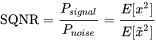
As shown in the above equation, we will measure the ratio of signal power to noise power. This representation applied on log scale converts to dB (10log10SQNR). Here signal is floating point input which we are quantizing to nearest integer and noise is Quantization noise. example: The elephant example of input has maximum value of 131.32, but we are representing this to nearest integer possible, which is 127. Hence it makes Quantization noise = 131.32–127 = 4.32.So SQNR = 131.32² /4.32² = 924.04, which is 29.66 db, indicating that we have only attained close to 30dB as compared to 48dB (6*no_of_bits) possibility.

如上式所示，我们将测量信号功率与噪声功率之比。 应用于对数刻度的此表示形式转换为dB(10log10SQNR)。 这里信号是浮点输入，我们将其量化为最接近的整数，而噪声是量化噪声。 示例 ：输入的大象示例的最大值为131.32，但我们将其表示为可能的最接近整数，即127。因此，它使量化噪声= 131.32–127 = 4.32。因此SQNR =131.32²/4.32²= 924.04，这是29.66 db，表明与48dB(6 * no_of_bits)可能性相比，我们仅达到了近30dB。

This reflection of SQNR on accuracy can be established for each individual network depending on structure. But indirectly we can say better the SQNR the higher is the accuracy.

可以根据结构为每个单独的网络建立SQNR对准确性的反映。 但是间接地，我们可以说SQNR越好，准确性就越高。

量化环境中的卷积： (Convolution in Quantized environments:)

The convolution operation in CNN is well known, where we multiply the kernel with input and accumulate to get the results. In this process we have to remember that we are operating with 8 bits as inputs , hence the result of multiplication need at least 16 bits and then accumulating it in 32 bits accumulator, which would help to maintain the precision of the result. Then result is rounded or truncated to 8 bits to carry 8 bit width of data.

CNN中的卷积运算是众所周知的，我们将内核乘以输入并累加以获得结果。 在此过程中，我们必须记住，我们使用8位作为输入，因此乘法结果至少需要16位，然后将其累加到32位累加器中，这将有助于保持结果的精度。 然后将结果舍入或截断为8位，以携带8位宽度的数据。

def conv_single_step_quantized(a_slice_prev, W, b,ip_fract,wt_fract,fract_dout):"""Apply one filter defined by parameters W on a single slice (a_slice_prev) of the output activationof the previous layer.Arguments:a_slice_prev -- slice of input data of shape (f, f, n_C_prev)W -- Weight parameters contained in a window - matrix of shape (f, f, n_C_prev)b -- Bias parameters contained in a window - matrix of shape (1, 1, 1)Returns:Z -- a scalar value, result of convolving the sliding window (W, b) on a slice x of the input data"""# Element-wise product between a_slice and W. Do not add the bias yet.s = np.multiply(a_slice_prev.astype('int16'),W) # Let result be held in 16 bit# Sum over all entries of the volume s.Z = np.sum(s.astype('int32')) # Final result be stored in int32.# The Result of 32 bit is to be trucated to 8 bit to restore the data path.# Add bias b to Z. Cast b to a float() so that Z results in a scalar value.# Bring bias to 32 bits to add to Z.Z = Z + (b << ip_fract).astype('int32')# Lets find out how many integer bits are taken during addition.# You can do this by taking leading no of bits in C/Assembly/FPGA programming# Here lets simulateZ = Z >> (ip_fract+wt_fract - fract_dout)if(Z > 127):Z = 127elif(Z < -128):Z = -128else:Z = Z.astype('int8')return Z

The above code is inspired from AndrewNg’s deeplearning specialization course, where convolution from scratch is taught. Then modified the same to fit for Quantization.

上面的代码灵感来自AndrewNg的深度学习专业课程，该课程教授从头开始的卷积。 然后将其修改为适合量化。

量化环境中的批次规范 (Batch Norm in Quantized environment)

As shown in Equation 1.4, we have modified representation to reduce complexity and perform the Batch normalization.The code below shows the same implementation.

如公式1.4所示，我们修改了表示形式以降低复杂度并执行Batch规范化。以下代码显示了相同的实现。

def calculate_bn(x,bn_param,Bn_fract_dout):      x_ip = x[0]
      x_fract_bits = x[1]      bn_param_gamma_s = bn_param[0][0]      bn_param_fract_bits = bn_param[0][1]      op = x_ip*bn_param_gamma_s.astype(np.int16) # x*gamma_s      # This output will have x_fract_bits + bn_param_fract_bits      fract_bits =x_fract_bits + bn_param_fract_bits      bn_param_bias = bn_param[1][0]      bn_param_fract_bits = bn_param[1][1]      bias = bn_param_bias.astype(np.int16)      # lets adjust bias to fract bits      bias = bias << (fract_bits - bn_param_fract_bits)      op = op + bias # + bias      # Convert this op back to 8 bits, with Bn_fract_dout as fractional bits      op = op >> (fract_bits - Bn_fract_dout)      BN_op = op.astype(np.int8)      return BN_op

Now with these pieces in place for Quantization inference model, we can see now the Batch norm impact on quantization.

现在将这些块用于量化推理模型，我们现在可以看到批处理规范对量化的影响。

结果 (Results)

The Resnet-50 trained with Imagenet is used for python simulation to quantize the inference model. From the above sections, we bind the pieces together to only analyze the first convolution followed by Batch Norm layer.

使用Imagenet训练的Resnet-50用于python仿真以量化推理模型。 从以上各节中，我们将片段绑定在一起，仅分析第一个卷积，然后分析Batch Norm层。

The convolution operation is the heaviest of the network in terms of complexity and also in maintaining accuracy of the model. So lets look at the Convolution data after we quantized it to 8 bits. The below figure on left hand side represents the convolution output of 64 channels (or filters applied) output whose mean value is taken for comparison. The Blue color is float reference and green color is Quantized implementation. The difference plot (Left Hand side) gives indication of how much variation exist between float and quantized one . The line drawn in that Difference figure is mean, whose value is around 4. which means we are getting on an average difference between float and Quantized values close to a value of 4.

就复杂性和维持模型的准确性而言，卷积操作是网络中最繁重的操作。 因此，在将卷积数据量化为8位之后，让我们看一下它。 下图左侧代表64个通道(或应用的滤波器)输出的卷积输出，取其平均值进行比较。 蓝色是浮动参考，绿色是Quantized实现。 差异图(左手侧)表示浮点数和量化的点之间存在多少差异。 在该差值图中绘制的线是平均值，其值在4左右。这意味着我们在float和Quantized值之间获得了接近于4的平均差。

Convolution and Batch Norm Outputs

卷积和批范数输出

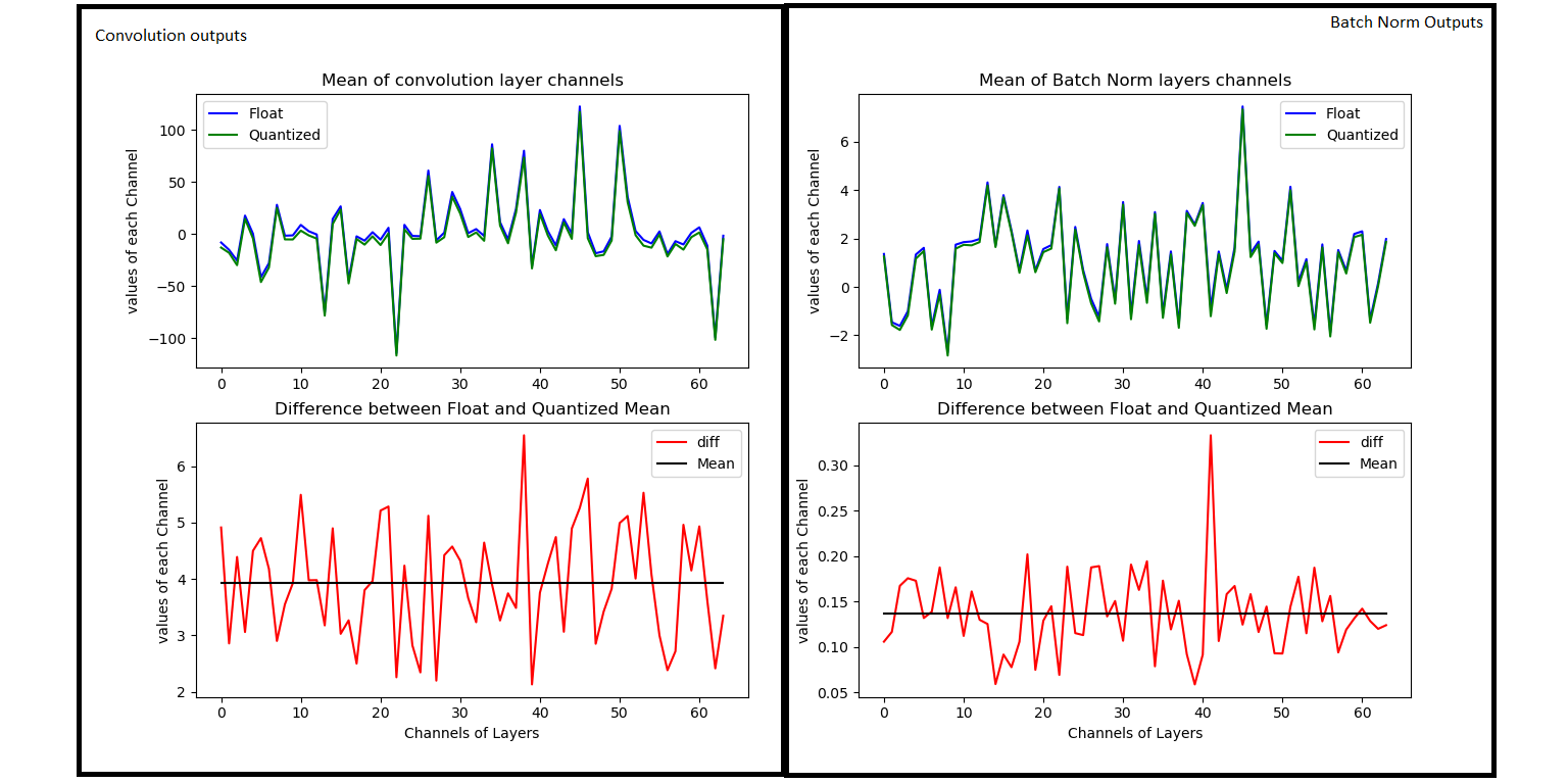
Now Lets look at Right Hand side figure, which is Batch Normalization section. As you can see the Green and blue curves are so close by and their differences range is shrunk to less than 0.5 range. The Mean line is around 0.135, which used to be around 4 in case of convolution. This indicates we are reducing our differences between float and quantized implementation from mean of 4 to 0.135(almost close to 0).

现在，让我们看一下右侧图，这是“批处理规范化”部分。 如您所见，绿色和蓝色曲线非常接近，它们的差异范围缩小到小于0.5的范围。 平均线约为0.135，在卷积情况下通常约为4。 这表明我们正在将浮点数和量化实现之间的差异从4的平均值减小到0.135(几乎接近0)。

Now Lets look at the SQNR plot to appreciate the Batch Norm impact.

现在，让我们看一下SQNR图，以了解批处理规范的影响。

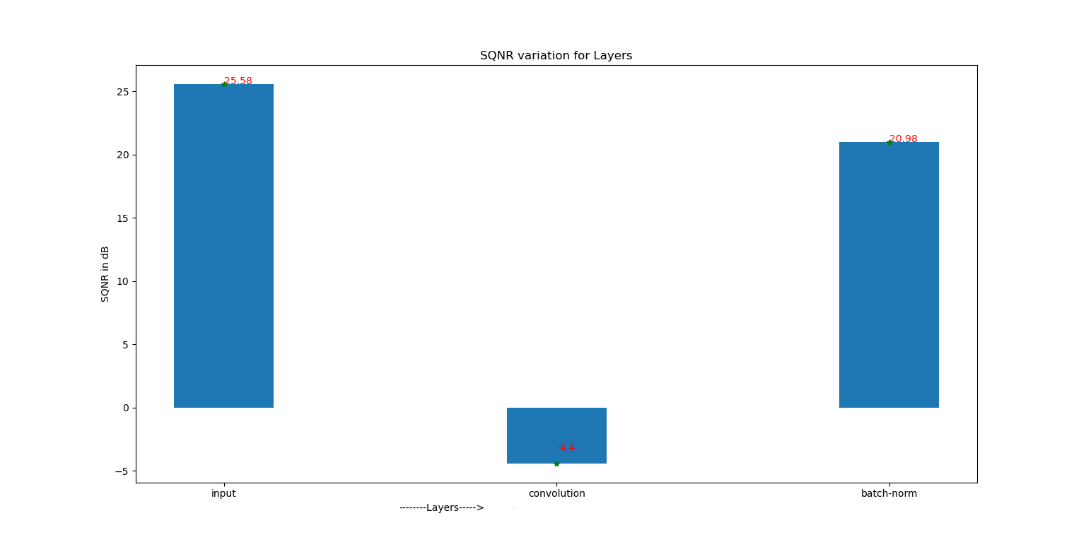
Just in case values are not visible, we have following SQNR numbers Input SQNR : 25.58 dB (The Input going in to Model)Convolution SQNR : -4.4dB (The output of 1st convolution )Batch-Norm SQNR : 20.98 dB (The Batch Normalization output)

以防万一值不可见，我们有以下SQNR编号输入SQNR：25.58 dB(输入模型输入)卷积SQNR：-4.4dB(第一次卷积的输出)批处理标准SQNR：20.98 dB(批量归一化)输出)

As you can see the input SQNR is about 25.58dB , which gets reduced to -4.4 dB indicating huge loss here, because of limitation in representation beyond 8 bits. But the Hope is not lost, as Batch normalization helps to recover back your SQNR to 20.98 dB bringing it close to input SQNR.

如您所见，输入SQNR约为25.58dB，由于表示限制超过8位，因此降低到-4.4 dB表示此处存在巨大损耗。 但是希望并没有失去，因为批量归一化有助于将SQNR恢复到20.98 dB，使其接近输入SQNR。

结论 (Conclusion)

• Batch Normalization helps to correct the Mean, thus regularizing the quantization variation across the channels.
  批量归一化有助于校正均值，从而规范化通道之间的量化变化。
• Batch Normalization recovers the SQNR. As seen from above demonstration, we see a recovery of SQNR as compared to convolution layer.
  批归一化恢复SQNR。 从上面的演示可以看出，与卷积层相比，我们看到了SQNR的恢复。
• If the quantized inference model on edge is desirable, then consider including Batch Normalization as it acts as recovery of quantization loss and also helps in maintaining the accuracy, along with training benefits of faster convergence.
  如果需要边缘上的量化推理模型，则应考虑包括“批归一化”，因为它既可以恢复量化损失，也可以帮助保持准确性以及更快收敛的训练好处。
• Batch Normalization complexity can be reduced by using (1.4), so that many parameters can be computed offline to reduce load on edge device.
  批处理规范化的复杂度可以通过使用(1.4)降低，以便可以离线计算许多参数以减少边缘设备的负载。

翻译自: https://medium.com/@vinaybk/batch-normalization-a-different-perspective-from-quantized-inference-model-7b1875681aa0