vecm
The outbreak of COVID-19 has caused unprecedentedly negative impacts across all industries, with manufacturing among the most suffered. At the second quarter of 2020, the US Industrial Production Index falls by 14.4% year-on-year. Shrinkage in industrial production is likely to create a negative demand shock for the input resources, which in turn drives down the prices of commodities, especially energy and metals.
COVID-19 吨他的爆发已经引起各个行业前所未有的负面影响,与其中最受到制造。 到2020年第二季度,美国工业生产指数同比下降14.4%。 工业生产的下降很可能会对投入资源产生负面的需求冲击,进而压低商品,特别是能源和金属的价格。
At the same time, variations in commodity prices would also affect the supply, production costs, and hence production decision. For example, the tentative agreement in April 2020 between the Organization of the Petroleum Exporting Countries (OPEC), Russia and other countries to extend oil production cuts aims to support oil price after a slump in demand caused by coronavirus lockdowns.
同时,商品价格的变化也会影响供应,生产成本,进而影响生产决策。 例如,石油输出国组织(OPEC),俄罗斯和其他国家在2020年4月达成的延长石油产量削减的暂定协议旨在在冠状病毒封锁导致需求下降之后支持石油价格。
Nonetheless, relationships among energy and metal prices could be even more complicated, not only due to their multi-directional linkages, but also due to the existence of time lagged effects, short run and long run equilibrium. In this article, I would try to apply Vector Error Correction Model (VECM) to (1) investigate the relationships between commodity prices and industrial production in the United States, and (2) forecast the movement of industrial production and commodity prices in near future. For all the codes below, please refer to my Github link here.
尽管如此,能源和金属价格之间的关系可能更加复杂,这不仅是因为它们之间存在多方向联系,而且还因为存在时间滞后效应,短期和长期均衡。 在本文中,我将尝试将向量误差校正模型(VECM)应用于(1) 研究美国商品价格与工业生产之间的关系 ,以及(2) 预测近期内工业生产和商品价格的变动 。 对于以下所有代码,请在此处参考我的Github链接。
数据 (Data)
大体时间 (Time Frame)
This exercise will focus on the period between January 1990 and July 2020.
这项工作的重点是1990年1月至2020年7月。
商品价格数据 (Commodities Price data)
From the World Bank’s commodity markets website, we can download the monthly price data for different commodities. Among all, below are selected as representatives of energy, industrial metals and precious metals.
从世界银行的商品市场网站上 ,我们可以下载不同商品的月度价格数据。 其中,以下是能源,工业金属和贵金属的代表。
Energy — Crude Oil (Brent), Coal (South African), Natural gas (US)
能源 -原油(布伦特),煤炭(南非),天然气(美国)
Industrial metals — Aluminum, Iron ore, Copper
工业金属 —铝,铁矿石,铜
Precious metals — Platinum, Silver
贵金属 -铂,银

As a side note, in 2019, the two traditional energy sources, e.g. petroleum and natural gas, still account for 74.0% of total energy use in the US industrial sector, which is a record high since data available in 1950. In contrast, only 9.5% in total is contributed by renewable energy, a slight decline from the peak of 10.1% in 2011. What a sad situation!!!
顺带一提, 在2019年,石油和天然气这两种传统能源仍占美国工业部门总能源消耗的74.0%,创下自1950年数据以来的最高记录 。 相比之下, 可再生能源仅贡献了9.5%,比2011年的10.1%的峰值略有下降 。 多么可悲的情况!!!

工业生产指数数据 (Industrial Production Index data)
For the United States’ industrial production index, data can be downloaded from the website of Federal Reserve Bank.
对于美国的工业生产指数,可以从联邦储备银行的网站下载数据。
According to the definition, the Industrial Production Index is an economic indicator that measures real output for all facilities located in the United States manufacturing, mining, and electric, and gas utilities (excluding those in U.S. territories).
根据定义, 工业生产指数是一种经济指标,用于衡量位于美国的制造,采矿,电力和天然气公用事业(不包括美国境内的所有设施)的所有设施的实际产出 。

矢量误差校正模型(VECM) (Vector Error Correction Model (VECM))
介绍 (Introduction)
Economic theory suggests that long run equilibrium exists between economic variables in their levels, which can render these variables stationary without taking differences, and this is so-called cointegration.
Ëconomic理论认为,在他们的水平的经济变量,它可以使这些变量固定不考虑差异之间存在长期均衡,这就是所谓的协整关系 。
Vector error correction model (VECM) serves as a way to capture such long run equilibrium relationships (levels) on top of short run relationships (differences). A more detailed explanation about VECM and its difference from Vector Autoregressive (VAR) model could be found here.
矢量误差校正模型(VECM)是一种在短期关系(差异)之上捕获此类长期均衡关系(水平)的方法。 在这里可以找到有关VECM及其与矢量自回归(VAR)模型的区别的更详细说明。
Prior to applying the VECM, let’s investigate whether the original time series data is stationary, which means that the variance of a time series is not dependent on time. If the time series is stationary, the plotted graph will look like a white noise.
在应用VECM之前,让我们研究原始时间序列数据是否稳定 ,这意味着时间序列的方差不依赖于时间。 如果时间序列是固定的,则绘制的图形将看起来像白噪声。
From the below line graph of non-differenced time series and correlation matrix, it’s likely that they are non-stationary, and there are cointegrations among them.
从下面的非差分时间序列和相关矩阵的折线图中,它们可能是不稳定的,并且它们之间存在协整。


无差异变量的自相关函数(ACF)分析 (Auto-Correlation Function (ACF) Analysis of Non-Differenced Variables)
Before proceeding, let’s take a look of the auto-correlation function plots of the 9 non-differenced time series, which show that they are definitely non-stationary.
在继续之前,让我们看一下9个非差分时间序列的自相关函数图,这些图表明它们确实是非平稳的。
#Test for stationary===========================================================
# plots the autocorrelation plots for each commodties price at 75 lags
for i in df:
    plot_acf(df[i], lags = 75)
    pyplot.title('ACF for %s' % i)
    pyplot.show()
变量自相关函数分析 (Auto-Correlation Function Analysis of Differenced Variables)
If we do the plot on variables after first difference, the ACFs of the differenced variables look potentially stationary. This suggests each time series is integrated I(1). Augmented Dickey-Fuller (ADF) tests can further confirm this.
如果我们对第一个差异后的变量进行绘图,则差异变量的ACF看起来可能是平稳的。 这表明每个时间序列都是积分的I(1)。 增强的Dickey-Fuller(ADF)测试可以进一步证实这一点。
#construct time series with first difference
df_diff = df.diff().dropna()


# plots the autocorrelation plots for the difference in each commodities price from the
# price the previous month at 75 lags
for i in df_diff:
    plot_acf(df_diff[i], lags = 75)
    pyplot.title('ACF for %s' % i)
    pyplot.show()
差分变量的增强Dickey-Fuller检验—平稳检验 (Augmented Dickey-Fuller Test for Differenced Variables — Test for stationary)
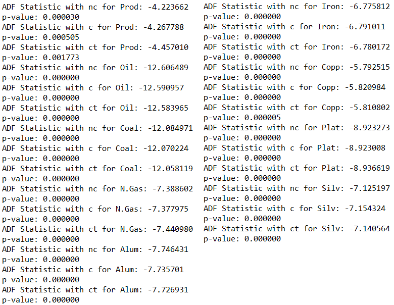
The null hypothesis is that the data are non-stationary. So if p-values are low, the data are stationary with high statistical significance.
零假设是数据是不稳定的。 因此,如果p值较低,则数据是固定的,具有较高的统计意义。
# performs the Augmented Dickey-Fuller Test for all our variables of interest without
# a constant, with a constant, and with a constant and linear trend
for i in df_diff:
    for j in ['nc', 'c', 'ct']:
        result = adfuller(df_diff[i], regression = j)
        print('ADF Statistic with %s for %s: %f' % (j, i, result[0]))
        print('p-value: %f' % result[1])
The results of the ADF tests for the differenced variables strongly support the hypothesis that the time series are integrated I(1). These time series need to be differenced once prior to modeling.
ADF检验差异变量的结果有力地证明了时间序列是积分I(1)的假设。 这些时间序列需要在建模之前进行一次差分。
Granger因果关系检验—因果关系检验 (Granger Causality Test — Test for causal relationships)
Next, we would like to see whether there are causal relationships between the time series through Granger causality test. The underlying story is that if previous values of X can predict future values of Y, then X Granger causes Y. An F-test is performed by estimating a regression of the lagged values of X on Y. If the p-value is small, we can reject the null hypothesis that all the coefficients of the lagged values of X are 0, i.e. lagged Xs have predictive power on future Y.
ñ分机,我们想看看是否有通过格兰杰因果检验时间序列之间的因果关系。 潜在的故事是,如果X的先前值可以预测Y的未来值,则X Granger会导致Y。F检验是通过估算X的滞后值在Y上的回归来进行的。如果p值很小,我们可以拒绝零假设,即X的所有滞后值的系数均为0,即,滞后X对未来Y具有预测能力。
#Granger Causality Test===========================================================
# creates a list of tuples containing the permutations of length 2
df_perms = list(permutations(df, 2))


# loops through the list of permutations
#for i in range(len(df_perms)):
for i in range(8):
    temp_list = list(df_perms[i])
    temp_df = df[temp_list]
    print('Does a lag of ' + temp_list[1] + ' predict ' + temp_list[0])
    print(grangercausalitytests(temp_df, maxlag = 3, addconst = True, verbose = True))
    print('')
    print('')
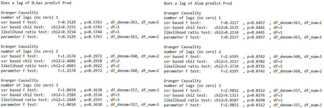
For simplicity, below only shows the test results on the US Industrial Production Index. The outputs show that all commodity prices, besides price of natural gas, have predictive power on the industrial production of the US. Therefore, it is appropriate for us to perform the VEC modelling after taking out the price of natural gas.
为简单起见,下面仅显示美国工业生产指数上的测试结果。 产出显示,除天然气价格外,所有商品价格均对美国的工业生产具有预测力。 因此,在扣除天然气价格之后,适合进行VEC建模。


Johansen协整测试—协整测试 (Johansen Cointegration Test — Test for cointegration)
In next step, we are going to test whether cointegration (long run) relationships exist between the time series by Johansen Cointegration Test.
在下一步中,我们将通过Johansen Cointegration Test检验时间序列之间是否存在协整(长期)关系。
#Johansen Cointegration test===================================================
def johansen_trace(y, p):
        N, l = y.shape
        joh_trace = coint_johansen(y, 0, p)
        r = 0
        for i in range(l):
            if joh_trace.lr1[i] > joh_trace.cvt[i, 1]:
                r = i + 1
        joh_trace.r = r
        return joh_trace


# loops through 1 to 6 lags of months
for i in range(1, 7):
    # tests for cointegration at i lags
    joh_trace = johansen_trace(df_selected, i)
    print('Using the Trace Test, there are', joh_trace.r, '''cointegrating vectors at
    %s lags between the series''' % i)
    print()
The results of this test show that there are 3 and 2 cointegrating relationships between the series at 1 and 2 lags respectively. Moreover, there is 1 cointegrating relationship between the time series at 3, 4, 5 and 6 lags during the sample period at the 95% significance level. Therefore, we can say that VEC modeling is appropriate to modeling these time series data.
该测试的结果表明,在1个滞后和2个滞后之间,序列之间分别存在3个和2个协整关系。 此外,在采样期间,在95%显着性水平的3、4、5和6个滞后时间序列之间存在1个协整关系。 因此,可以说, VEC建模适合于对这些时间序列数据进行建模 。

VECM估计和分析 (VECM Estimation & Analysis)
#Vector error corretion model (VECM)===========================================
# estimates the VECM on the closing prices with 6 lags, 1 cointegrating relationship, and
# a constant within the cointegration relationship
model_vecm = VECM(endog = df_selected, k_ar_diff = 6, coint_rank = 1, deterministic = 'ci')
model_vecm_fit = model_vecm.fit()
model_vecm_fit.summary()
The loading coefficients (alphas) represent how quickly the time series converge to the long-run equilibrium relationship.
加载系数(alpha)表示时间序列收敛到长期平衡关系的速度。
The alphas for prices of oil, coal, aluminum and silver are statistically significant at the 0.05 significance level, while those for prices of copper and platinum are significant at the 0.10 significance level. However, the alpha for the prices of iron ore is not statistically significant.
石油,煤炭,铝和银的价格的alpha值在0.05的显着性水平上具有统计学意义,而铜和铂金的价格的alpha值在0.10的显着性水平上显着。 但是,铁矿石价格的alpha值在统计上并不重要。
From the result, we know that price of iron ore is weakly exogenous to the US industrial production index. Weak exogeneity means that deviations from the long-run do not directly affect the weakly exogenous variable. The effect comes from the subsequent lags of those non-weakly exogenous variables. In other words, the lags of other commodity prices are the drivers of the return to the long-run equilibrium in the weakly exogenous variables (price of iron ore).
从结果可以看出,铁矿石价格对于美国工业生产指数而言是弱外生的。 弱的外生性意味着与长期的偏离不会直接影响弱外生变量。 影响来自那些非弱外生变量的后续滞后。 换句话说, 其他商品价格的滞后是弱外生变量(铁矿石价格)回归长期均衡的驱动力 。

The beta coefficients are the actual long-run relationship coefficients. The beta for the US Industrial Production Index is standardized at 1 for ease of interpretation of the other beta coefficients.
Beta系数是实际的长期关系系数。 美国工业生产指数的beta标准化为1,以便于解释其他beta系数。
Among all, the beta for silver price is -6.0521, which means that a 1 dollar increase in silver price would lead to a 6.0521 decrease in the US Industrial Production Index in the long-run. Similarly, the betas for prices of oil, coal and aluminum are -3.5384, -0.4791 and -0.0793.
其中,白银价格的beta是-6.0521,这意味着从长期看白银价格每增加1美元,美国工业生产指数将下降6.0521。 同样,石油,煤炭和铝价格的beta为-3.5384,-0.4791和-0.0793。
In contrast, the beta for iron ore price is 1.2618, which means that a 1 dollar increase in iron ore price would lead to a 1.2618 increase in the US Industrial Production index in the long run. Similarly, the betas for prices of platinum and copper are 0.1313 and 0.0334 respectively.
相比之下,铁矿石价格的beta为1.2618,这意味着从长远来看,铁矿石价格每上涨1美元,美国工业生产指数就会上涨1.2618。 同样,铂金和铜价的beta分别为0.1313和0.0334。
脉冲响应功能 (Impulse Response Function)
#Impulse response function=====================================================
irf = model_vecm_fit.irf(24)
irf.plot(orth = False)
Impulse Response Function (IRF) shows the response of one variable when another or the same variable is shocked with an increase of 1 unit in the previous period (month). The blue curve shows the effect of the unit shock when time passes, and the dotted lines represent the 95% confidence interval for the IRF. Here, we try to observe the impulse response for a period of 24 months.
脉冲响应函数(IRF)显示了一个变量在上一个期间(月)以1个单位的增加受到冲击时对另一个变量的响应。 蓝色曲线显示了时间流逝时单位电击的影响,虚线表示IRF的95%置信区间。 在这里,我们尝试观察24个月的脉冲响应。

Let’s focus on the IRF for the US Industrial Production Index.
让我们关注美国工业生产指数的IRF。
First, from the first column of the above graph, it’s interesting to see that if the Industrial Production Index experienced a shock with an increase of 1 unit in the previous month, the prices of all the commodities will rise. This observation could be supported by the logic of demand shocks.
首先,从上图的第一列中可以很有趣地看到, 如果工业生产指数在上个月增加1个单位后受到冲击,则所有商品的价格都会上涨。 需求冲击的逻辑可以支持这一观点。
Second, from the first row of the above graph, we can see that an one unit positive shock to the prices of oil, aluminum, iron, copper and silver would lead to a rise in industrial production, though in different extents and duration. The rationale behind could be a greater motivation for mining, electric and gas utilities industries to output amid rising commodity prices.
其次,从上图的第一行可以看出, 对石油,铝,铁,铜和白银的价格形成单一正面冲击将导致工业生产上升,尽管程度和持续时间不同。 背后的理由可能是在大宗商品价格上涨的情况下,采矿,电力和天然气公用事业行业更大的动力 。
Third, negative impacts are brought to the Industrial Production Index when prices of coal and platinum experience a positive shock of one unit. The rise in these commodity prices may lead to higher input costs to manufacturing sectors, and thus hinder industrial production.
第三, 当煤炭和铂金的价格受到一个单位的正冲击时 , 会对工业生产指数产生负面影响。 这些商品价格的上涨可能导致制造业的投入成本增加,从而阻碍工业生产。
You may observe that there could be two dominating but contradictive factors within the Industrial Production Index — manufacturing versus mining & utilities. Rise of a commodity price may encourage mining and utilities activities but slow down manufacturing.
您可能会发现,工业生产指数中可能存在两个主要但相互矛盾的因素-制造业,采矿业和公用事业。 大宗商品价格上涨可能会鼓励采矿和公用事业活动,但会拖慢制造业。
If we look at the IRF of other commodities, there are many interesting observations. For example, the one unit shock in oil price will generate negative impacts on coal price, and vice versa. A substitution effect may be illustrated. Therefore, it may be worthy to conduct in-depth investigation on the industrial use of each commodity and the relationships among them.
如果我们看一下其他商品的IRF,就会发现很多有趣的发现。 例如, 石油价格的一次冲击将对煤炭价格产生负面影响,反之亦然。 可以说明替代效果。 因此,有必要对每种商品的工业用途及其之间的关系进行深入研究。
动态预测 (Dynamic Forecasting)
#Dynamic forecasting===========================================================
model_vecm_fit.plot_forecast(12, n_last_obs=60)
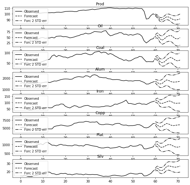
Last but not least, below is a dynamic forecasting graph of the US Industrial Production Index and commodity prices for upcoming one year.
最后但并非最不重要的是,下面是未来一年美国工业生产指数和商品价格的动态预测图。

In fact, the forecasts are in line with our expectations surprisingly.
实际上,这些预测出乎我们的意料。
(i) Industrial production is hard to pick up in short term, and may even decline slightly further. A strong recovery signal has not yet been sent from the US economy. The relatively weak trend is likely to continue for a longer period.
(i)短期内工业生产很难恢复,甚至可能进一步下降。 美国经济尚未发出强劲的复苏信号。 相对较弱的趋势可能会持续更长的时间。
(ii) Prices of all commodities besides silver will maintain at similar level. Demand, supply and geopolitics remain the fundamentals to affect commodity prices. Without some specific events, such as Russia — Saudi Arabia oil price war in March, the commodity prices tend to be stable.
(ii)除白银外,所有其他商品的价格将维持在相似的水平。 需求,供应和地缘政治仍然是影响商品价格的基本面。 没有三月的俄罗斯-沙特阿拉伯石油价格战等具体事件,大宗商品价格趋于稳定。
(iii) The current rising trend of silver price may continue. Besides industrial use, silver also serves as a store of value amid accommodative monetary policy.
(iii)当前白银价格的上涨趋势可能会继续。 除了工业用途,在宽松的货币政策下,白银还可以作为价值的存储。
结论 (Conclusion)
This article has made use of a popular econometric model — Vector Error Correction Model (VECM) to help us understand both the short run and long run relationships between the Industrial Production and different commodity prices. The model has successfully built up a linkage between the data and reality.
本文利用了流行的计量经济学模型— 矢量误差校正模型(VECM)来帮助我们了解工业生产与不同商品价格之间的短期和长期关系。 该模型已成功建立了数据与现实之间的联系。
Either the impulse response function or the dynamic forecasting is showing a result that is in line with our expectations and economic rationale. I hope this would raise your interests to analyze and forecast the economies through econometric modelling.
脉冲响应函数或动态预测所显示的结果都符合我们的预期和经济原理。 我希望这会引起您的兴趣,以便通过计量经济学建模来分析和预测经济。
Thank you very much. See you next time.
非常感谢你。 下次见。
vecm


 本文通过应用向量误差修正模型(VEC模型)探讨了商品价格变化如何影响美国的工业生产。通过对数据进行分析,揭示两者之间的动态关系。


 2158
2158

 被折叠的 条评论
为什么被折叠?


