


总览 (Overview)
My next analysis was inspired from various baseball-industry related experiences. Before pursuing my graduate degree, I had numerous jobs working in baseball, specifically in the player evaluation/scouting sector. As such, I learned that when evaluating an amateur pitching prospect, there are many things to keep in mind, including:
我的下一个分析是从与棒球行业有关的各种经验中获得启发的。 在攻读研究生学位之前,我曾在棒球领域从事很多工作,特别是在球员评估/球探领域。 因此,我了解到,在评估业余投球前景时,需要牢记许多事情,包括:
- Player Age 球员年龄
- Athleticism Traits 运动特质
- Data points such as spin rate, velocity, horizontal and vertical break, etc.. 数据点,例如旋转速度,速度,水平和垂直断裂等。
- Competition Level 比赛水平
- Body Type 体型
With this said, traditional player evaluation typically stems from human observation. In other words, how is this player special from the traits that can be observed by the human eye? This process has worked effectively since the inception of the game. This got me thinking, however, is there a way we can quantify a baseline for a prospect? While we generally know what traits are important, can we determine which are more important than others? This lead me down an interesting path that resulted in some insightful conclusions.
话虽如此,传统的玩家评估通常源于人类的观察。 换句话说,从人眼可以观察到的特征来看,这个玩家有何特别之处? 自游戏开始以来,此过程一直有效。 但是,这让我开始思考,是否有一种方法可以量化潜在客户的基准? 虽然我们通常知道哪些特征很重要,但是我们可以确定哪些特征比其他特征更重要吗? 这引导我走了一条有趣的道路,得出了一些有见地的结论。
数据 (The Data)
For this project, I utilized two data sources: Baseball Savant and the Lahman Database. If you are familiar with my past articles or are a baseball fan in general, I am sure you have heard of Baseball Savant. The Lahman database is less-widely used by the general public but contains some incredibly helpful data. While the database has information on a diverse set of topics such as traditional statistics, player awards, and general team info, I used it for biographical data.
对于这个项目,我利用了两个数据源: Baseball Savant和Lahman Database 。 如果您熟悉我的过往文章,或者是一般的棒球迷,那么我相信您已经听说过“棒球狂人”。 Lahman数据库在公众中使用的范围较广,但其中包含一些非常有用的数据。 虽然数据库包含有关各种主题的信息,例如传统统计数据,球员奖励和一般球队信息,但我将其用于个人资料。
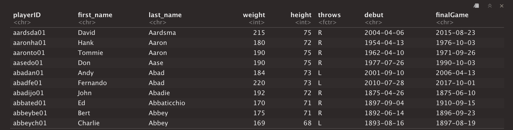
The Lahman database provides the user many different connection options, one being an R-Studio package that provides access to all of its capabilities. Below is a snippet of the data gathered from the Lahman database.
Lahman数据库为用户提供了许多不同的连接选项,其中一个是R-Studio程序包,可以访问其所有功能。 以下是从拉曼数据库中收集的数据片段。
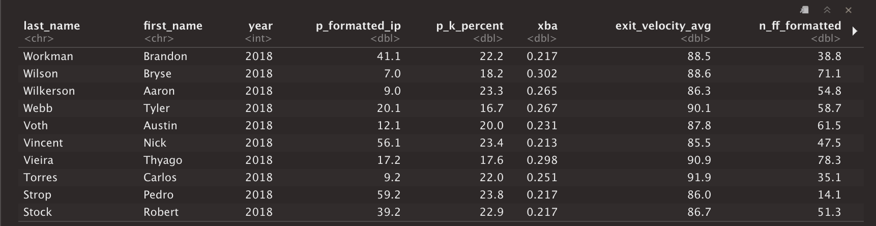
Regarding the Baseball Savant data, my primary goal was to extract pitch arsenal related information, in addition to a few modern statistics that will be utilized in my success metric (which I will get into later). Here is a quick guide to the pitch arsenal features pulled in addition to the metrics used in my success feature:
关于“棒球狂热”数据,我的主要目标是提取与球场阿森纳相关的信息,以及一些将用于我的成功度量标准的现代统计数据(稍后将介绍)。 除了成功功能中使用的度量标准外,这还提供了有关推销球场武库功能的快速指南:
Arsenal Data:
阿森纳数据:
- Pitch Type 螺距类型
- Percent Thrown (per pitch type) 投掷百分比(每个音高类型)
- Velocity (per pitch type) 速度(每个音高类型)
- Spin (per pitch type) 旋转(每节距类型)
- Horizontal and Vertical Break (per pitch type) 水平和垂直折断(按螺距类型)
- Total Break (per pitch type) 总间隔(每个音高类型)
Metrics:
指标:
- Innings Pitched 因宁投球
- K% K%
- xBA xBA
- Exit Velocity 出口速度
数据处理 (Data Processing)
In order to transform the data into a structure that is optimal for the questions I am trying to answer, a great deal of processing was needed. This was by far the most time consuming portion of this analysis and required multiple steps. In order to provide a clear layout of my strategy, I will break each processing portion into a descriptive step.
为了将数据转换为最适合我尝试回答的问题的结构,需要进行大量处理。 到目前为止,这是此分析中最耗时的部分,需要多个步骤。 为了提供清晰的战略布局,我将每个处理部分分成一个描述性步骤。
Step 1: Merge the Lahman and Savant Data
步骤1 :合并Lahman和Savant资料
This step was relatively simple. Once I identified a feature prevalent in both the savant and lahman data sets, they were aggregated into one master group. Since they both contained a variable with each player’s first and last name, this was a relatively straightforward step.
此步骤相对简单。 一旦我确定了savant和lahman数据集中都存在的特征,就将它们汇总到一个主组中。 由于它们都包含一个变量,每个变量都有每个玩家的名字和姓氏,因此这是一个相对简单的步骤。
Step 2: Average Out Repeated Player Data
步骤2:平均淘汰重复玩家资料
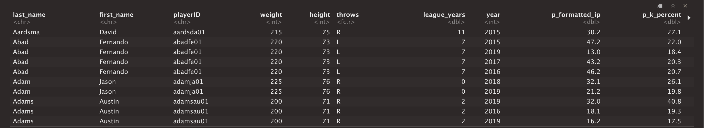
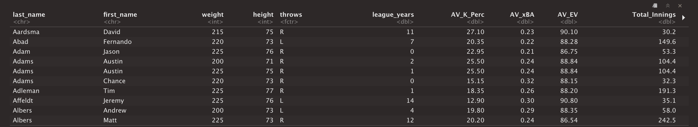
Now that the master set was created, I had to determine how I was going to deal with repeated player seasons. Since the savant data tracks metrics from 2015 and on, there were many players that participated in seasons 2015–2020. As a result, I needed to average out their metrics, creating one observation per player, rather than an observation per season of each player. An example of this process is found below. Specifically, compare the top table “Fernando Abad” observations to the newly transformed table below.
既然已经创建了大师赛,我必须确定如何应对重复的球员赛季。 由于savant数据跟踪了2015年及以后的指标,因此有很多参与者参与了2015-2020赛季。 结果,我需要对他们的指标进行平均,从而为每个玩家创建一个观察值 ,而不是每个赛季的观察值 。 以下是此过程的示例。 具体来说,将顶部表格“ Fernando Abad”的观察结果与下面新转换的表格进行比较。
Step 3: Create a ‘Success’ Feature
第3步 :创建“成功”功能
In order to create the ideal prospect, I needed to create some sort of baseline of characteristics to look for. While there are a wide variety of paths I could have chosen, I based my success metric off of the following variables: AV_K_Perc, AV_xBA, AV_EV, and Total_Innings. Now that the variables are selected, I needed some sort of threshold that would classify a player as successful or unsuccessful.
为了创造理想的前景,我需要创建某种形式的特征基线来寻找。 尽管可以选择多种路径,但我的成功指标基于以下变量: AV_K_Perc,AV_xBA,AV_EV和Total_Innings 。 现在已经选择了变量,我需要某种阈值来将玩家分类为成功还是失败。
In order to do so, I simply looked at league averages, determining what quantile the player would need to fall under in order to be considered successful. This fangraphs article was incredibly useful and was the driving force in determing the overall thresholds. My final thresholds were as follows:
为了做到这一点,我只是查看了联盟的平均值,确定了要想获得成功,球员需要落在哪个分位数上。 这篇带有幻想的文章非常有用,并且是确定总体阈值的推动力。 我的最终阈值如下:
- K% ≥= 22 K%≥= 22
- xBA ≤ .240 xBA≤.240
- EV ≤ 88 EV≤88
- Total Innings ≥ 80 总局限≥80
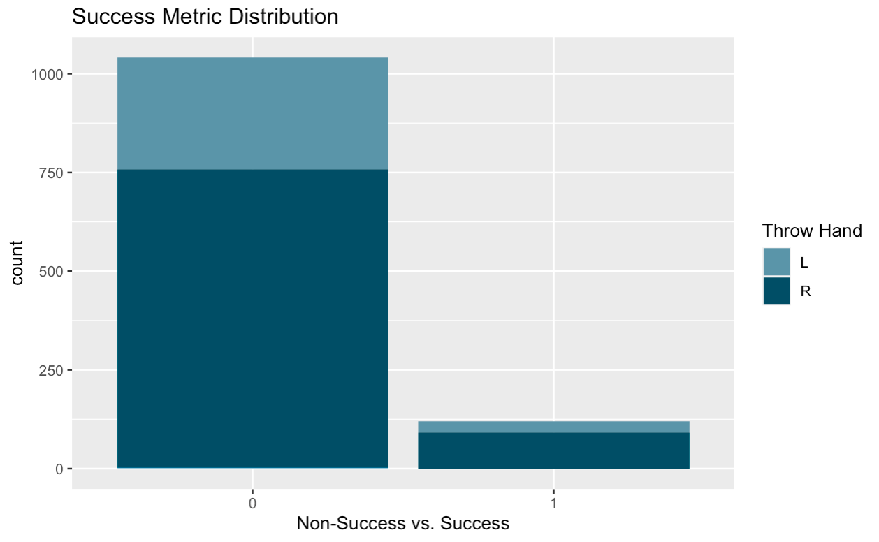
Now that these metrics were decided, I created a new binary feature in the data named ‘success’ that identifies a player as successful (1) or unsuccessful (0). It is key to note that in order for the player to be considered successful, EACH threshold must be met.
现在确定了这些指标之后,我在名为“成功”的数据中创建了一个新的二进制功能,该功能将玩家识别为成功(1)或不成功(0)。 关键要注意的是,为了使玩家被认为是成功的,必须满足每个阈值。
Step 4: Use cut2 Function to Put Data Into Quantiles
步骤4 :使用cut2函数将数据放入分位数
Similarly to the ‘success’ feature created above, I needed to continue the process with the majority of other variables present in the data. Before I could do so, I needed to seperate the data into quantiles.
与上面创建的“成功”功能类似,我需要使用数据中存在的大多数其他变量来继续该过程。 在这样做之前,我需要将数据分成几分位数。
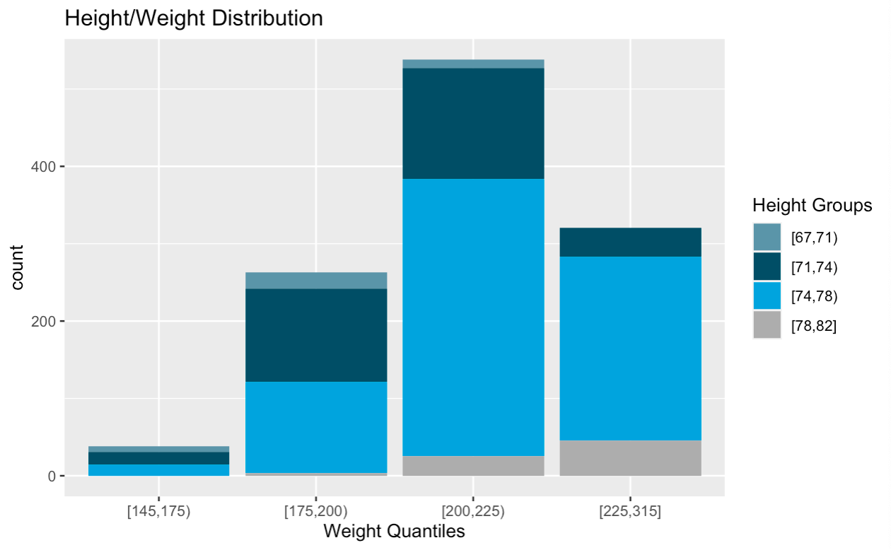
For example, the data contained players with heights ranging from 67–78 inches. To have the capability to determine the optimal height, ranges are required. As such, I split the height variable into the following 4 quantiles: 67–70, 71–73, 74–78. The identical process was required for ALL other variables including each individual pitch’s metrics.
例如,数据包含身高在67-78英寸之间的球员。 为了具有确定最佳高度的能力,需要范围。 因此,我将高度变量分为以下4个分位数:67-70、71-73、74-78。 所有其他变量(包括每个音高的指标)都需要相同的过程。
Step 5: Create Binary Variables for Each Cut Quantile
步骤5 :为每个切割的分位数创建二进制变量
The final data processing step required me to take each quantized variable and create its own unique variable based on its value. To explain this, I will use the weight variable. Before the binary creation, the weight variable classified each observation in a specific quantile.
最后的数据处理步骤要求我获取每个量化变量,并根据其值创建自己的唯一变量。 为了解释这一点,我将使用weight变量。 在创建二进制文件之前,权重变量将每个观察值分类为特定的分位数。
For example, say player A weighs 210 pounds. Since 210 falls between 200–224, player A has a value of [200,225) in the weight variable. In order to analyze this, I needed to create a binary variable for the [200,225) observations, specifically named ‘weight_200_224’. If a player’s weight falls within this category, a ‘1’ will be utilized as the value, with a ‘0’ otherwise.
例如,假设玩家A重210磅。 由于210介于200-224之间,因此玩家A的权重变量的值为[200,225)。 为了对此进行分析,我需要为[200,225)个观测值创建一个二进制变量,专门命名为'weight_200_224'。 如果玩家的体重在此类别之内,则将使用“ 1”作为值,否则使用“ 0”。
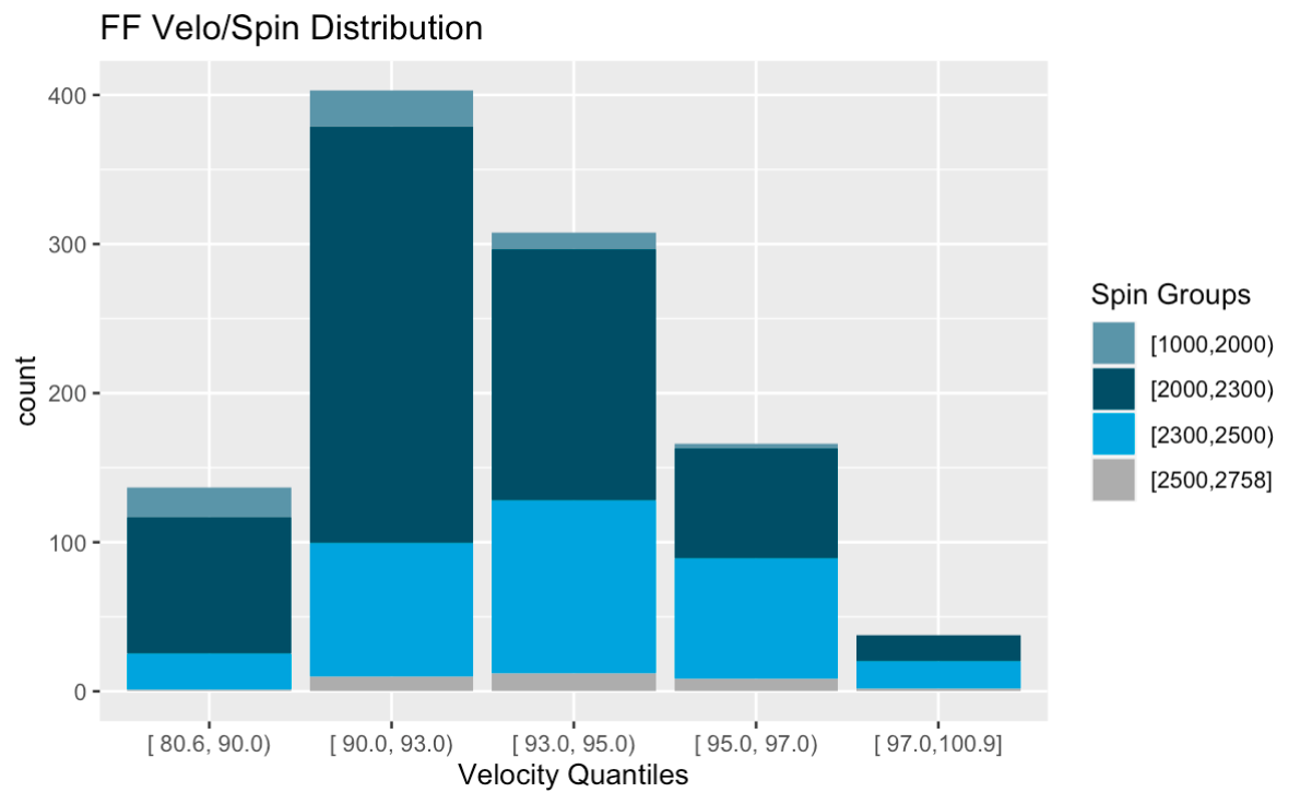
While this may seem like a simple example, there were a ton of instances where this process needed to take place. Take the four seam fastball velocity metric as an example. The following variables were created for FF velocity: ff_velo_80_89, ff_velo_90_92, ff_velo_93_94, ff_velo_95_96, ff_velo_97_plus.
尽管这似乎是一个简单的示例,但是有很多实例需要执行此过程。 以四个接缝快球速度度量为例。 为FF速度创建了以下变量:ff_velo_80_89,ff_velo_90_92,ff_velo_93_94,ff_velo_95_96,ff_velo_97_plus。
功能重要性-最佳武器库 (Feature Importance — Optimal Arsenal)
Now that the data is split into quantiles with unique binary variables per quantile, the data is ready for analysis, leading into the first question I aimed to answer: what is the optimal arsenal for a pitcher?
现在将数据分为每个分位数具有唯一二进制变量的分位数,现在可以对数据进行分析了,这是我要回答的第一个问题:投手的最佳武库是什么?
By utilizing the newly created success metric, I ran a random forest algorithm to determine feature importance. For this model, I created a data.frame containing only the success metric in addition to each binary pitch type variable.
通过利用新创建的成功指标,我运行了一个随机森林算法来确定特征的重要性。 对于此模型,我创建了一个data.frame,除了每个二进制音高类型变量之外,仅包含成功指标。
From here, I was able to determine what pitches have the highest impact on overall success. The model resulted in some pretty interesting findings, which can be found below.
从这里,我能够确定哪些策略对整体成功有最大的影响。 该模型产生了一些非常有趣的发现,可以在下面找到。
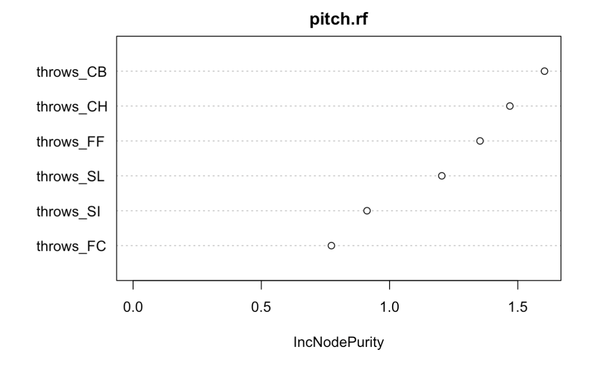
In order to corroborate these observations, I created a correlation matrix, aiming to identify the variables that have the highest correlation with success. As you can see below, the matrix agreed that throwing a CB and CH have the highest impact on success.
为了证实这些观察结果,我创建了一个相关矩阵,旨在确定与成功相关性最高的变量。 正如您在下面看到的,矩阵同意,投掷CB和CH对成功的影响最大。
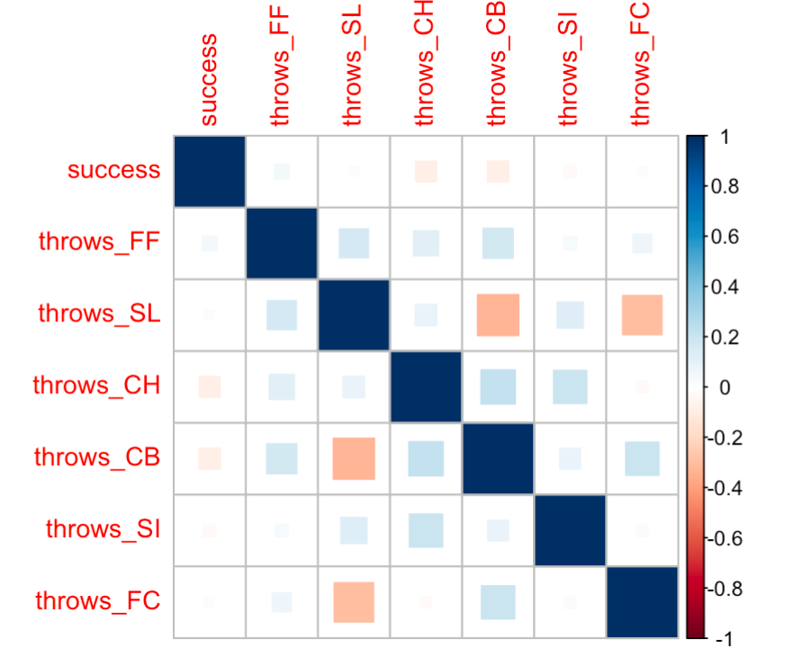
Based off the model and correlation matrix, a pitcher who throws both a CB and CH has the highest probability of success. Now that the optimal arsenal has been identified, I went ahead and subsetted the data based off pitchers who threw these pitches, resulting in the following groups:
根据模型和相关矩阵,投掷CB和CH的投手成功的可能性最高。 既然已经确定了最佳武器库,我继续根据投掷这些投球的投手对数据进行了子集化,结果分为以下几组:
- Pitchers who throw a CB, CH, FF (optimal) 投手投出CB,CH,FF(最佳)的投手
- Pitchers who throw a CB, CH, FF, SL 投手投出CB,CH,FF,SL的投手
创造最佳的投球前景 (Creating the Optimal Pitching Prospect)
Now that the arsenals are created, I conducted a similar process using all of the binary variables created in the data processing section. Below you will find the results of each one of the arsenals, as well as a summary for the optimal pitching prospect. If you would like to see ALL the recommended features for each aresenal type, they can be found here.
现在已经创建了武库,我使用在数据处理部分中创建的所有二进制变量进行了类似的过程。 在下面,您将找到每个武库的结果以及最佳投球前景的摘要。 如果您想查看每种军械库类型的所有推荐功能,请在此处找到。
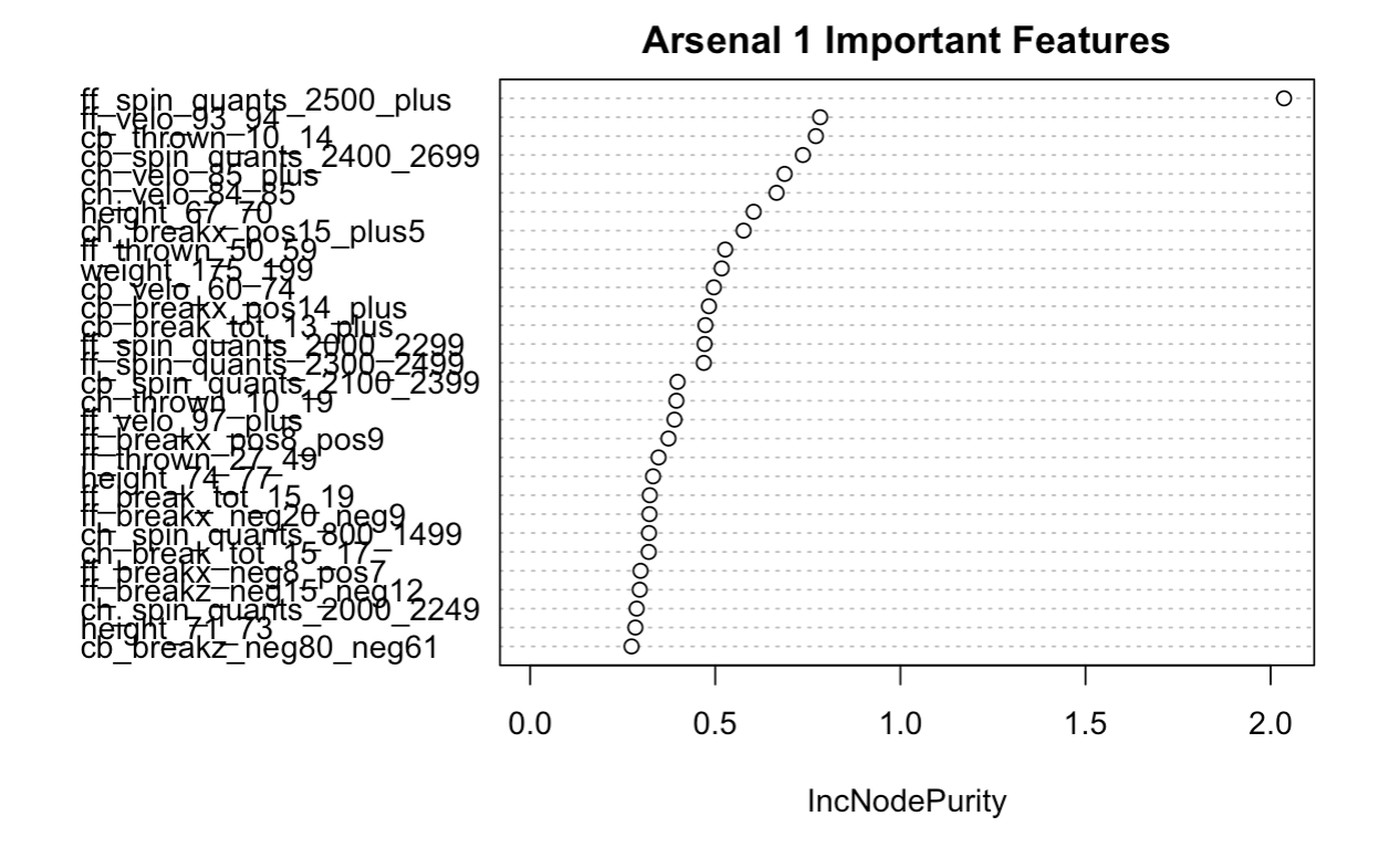
Arsenal 1: A Prospect Who Throws a FF, CB, CH (optimal)
阿森纳1 :投掷FF,CB,CH的准球员(最佳)
Key Characteristics:
主要特点:
- Four-Seam fastball spin of 2500 RPMS + 2500 RPMS的四缝快球旋转+
- Four-Seam fastball velocity between 93–94 MPH 93-94 MPH之间的四缝快球速度
- Curveball thrown 10–14 % of the time 曲线球投掷10–14%的时间
- Height between 67–70 inches 高度介于67-70英寸之间
- Weight between 175–199 pounds 重量在175-199磅之间
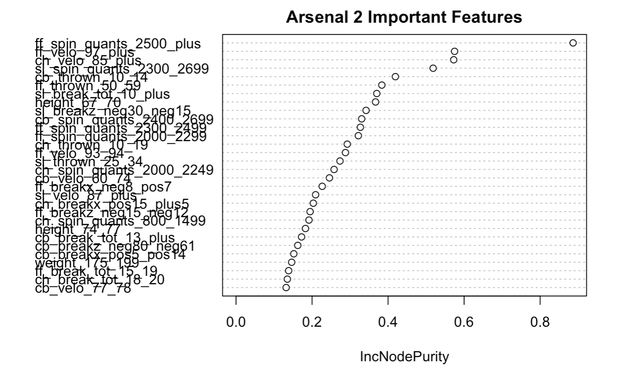
Arsenal 2: A Prospect Who Throws a FF, CB, CH, SL
阿森纳2 :投掷FF,CB,CH,SL的前景
Key Characteristics:
主要特点:
- Four-Seam fastball spin of 2500 RPMS + 2500 RPMS的四缝快球旋转+
- Four-Seam fastball velocity 97 MPH + 四缝快球速度97 MPH +
- Changeup velocity 85 MPH + 转换速度85 MPH +
- Slider total break of 10 inches + 滑块总断裂10英寸+
结论 (Conclusions)
There were a lot of questions answered throughout this analysis. Here are a few findings.
在整个分析过程中,回答了很多问题。 以下是一些发现。
The impact of a high spin fastball
高旋转快球的影响
This feature, above all else, should be considered the most important factor in evaluating players. If a pitcher has a spin of 2500+, there is a good chance he will be able to succeed.
首先,此功能应被视为评估玩家的最重要因素。 如果投手的旋转角度为2500+,那么他很有可能会成功。
2. Curveballs!
2. 曲线球!
This can be a difficult subject. As research has concluded, including another one of my personal projects, breaking balls increase the chance of UCL injuries.
这可能是一个困难的课题。 研究结束时,包括我的另一个个人研究项目 ,打破球会增加UCL受伤的机会。
It’s also interesting to note that while curveballs are the most important pitch, the model concluded they should only be thrown 10–14% of the time.
有趣的是,虽然弯球是最重要的投球,但模型得出的结论是,投掷球的时间应该只有10%至14%。
改进之处 (Improvements)
This was a fun and interesting project. However, there are multiple areas that it can improve, beginning with:
这是一个有趣而有趣的项目。 但是,它可以从多个方面改进:
Data, data, data
数据,数据,数据
After all the data processing, the master set contained just over 1000 variables. The main limitation here was that Statcast data is only tracked from 2015-on. As such, there are only so many players to work with, limiting the overall scope of the analysis.
经过所有数据处理后,主集中仅包含1000多个变量。 这里的主要限制是仅从2015年起才跟踪Statcast数据。 因此,只有太多的参与者可以合作,从而限制了分析的总体范围。
2. Can’t Account for Projectability
2.无法说明可投影性
While the goal was to use the ‘success’ metric to help evaluate amateur players, the reality is that the player at 18 years old won’t be the same player at 23 years old. There is a ton of development time that occurs throughout those crucial years and are not accounted for in this analysis.
虽然目标是使用“成功”指标来帮助评估业余玩家,但现实情况是18岁的玩家不会是23岁的玩家。 在那些关键的年份中有大量的开发时间,在此分析中并未考虑。
3. Height/Weight Distribution
3.身高/体重分布
While the height/weight data was interesting to include, it is important to note the data stems from when the player first entered the league. As a result, these biographical features (especially weight) are probably slightly different than the player’s current weight.
包括身高/体重数据是很有趣的,但重要的是要注意数据来自于球员首次进入联赛的时间。 结果,这些传记特征(尤其是体重)可能与玩家当前的体重略有不同。


 1890
1890

 被折叠的 条评论
为什么被折叠?
被折叠的 条评论
为什么被折叠?
 到【灌水乐园】发言


