


机器学习 客户流失
**Short code snippets and visualizations will be shared throughout this post but all the code for this project can be found in this Github Repo.
**简短的代码片段和可视化将在本文中共享,但是该项目的所有代码都可以在Github Repo中找到。
Companies put a lot of emphasis on customer acquisition, and rightfully so: companies need customers. However, customer acquisition costs are usually fairly high, and companies sometimes focus too much on acquisition and not enough on retention. A company may have great acquisition rates, but, if you also have a high Churn rate, you are essentially flushing those acquisition costs down the drain. The goal of this project is to demonstrate how machine learning can be used to identify customers who are likely to Churn in the coming months. If customers at high risk of Churn can be identified early, interventions can be done to retain that customer.
公司非常重视客户的获取,这是正确的:公司需要客户。 但是,客户获取成本通常很高,并且公司有时过多地专注于获取,而对保留率却不够。 公司的收购率可能很高,但是,如果客户流失率也很高,则实际上是在浪费这些收购成本。 该项目的目的是演示如何使用机器学习来识别未来几个月可能流失的客户。 如果可以及早发现客户流失风险高的客户,则可以采取干预措施挽留该客户。
What is Churn?
什么是客户流失?
If a customer cancels their service with your company, that is considered a Churn case.
如果客户取消了与您公司的服务,则视为“流失”案。
数据 (The Data)
For this project, I chose to use a dataset from a mobile phone carrier. The dataset contains information on 3,100 randomly selected customers. After cleaning, the dataset looks like this…
对于这个项目,我选择使用手机运营商的数据集。 该数据集包含有关3,100个随机选择的客户的信息。 清理后,数据集看起来像这样……
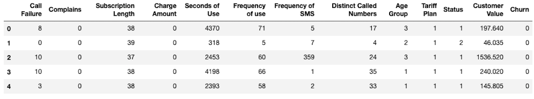
Each row represents a customer and each customer has 12 attributes associated with them as well as a 13th attribute (‘Churn’) that describes whether or not that customer canceled their service. Except for Churn, each attribute is an aggregate of 9 months of data (months 1–9). Churn is a record of whether or not that customer canceled service during months 9 through 12.
每行代表一个客户,每个客户都有与之关联的12个属性以及描述该客户是否取消其服务的第13个属性(“搅动”)。 除“客户流失”外,每个属性均汇总了9个月的数据(第1-9个月)。 客户流失记录是该客户在9到12个月内是否取消服务的记录。
Why do we need to predict Churn if there is already a Churn column?
如果已经有一个Churn列,为什么我们需要预测Churn?
We only have a Churn column because this is past data. We will use this past data to build a model, which can then be used on current data to predict Churn before it happens.
我们只有一个Churn列,因为这是过去的数据。 我们将使用过去的数据来构建模型,然后将其用于当前数据以预测流失。
可视化数据 (Visualizing the Data)
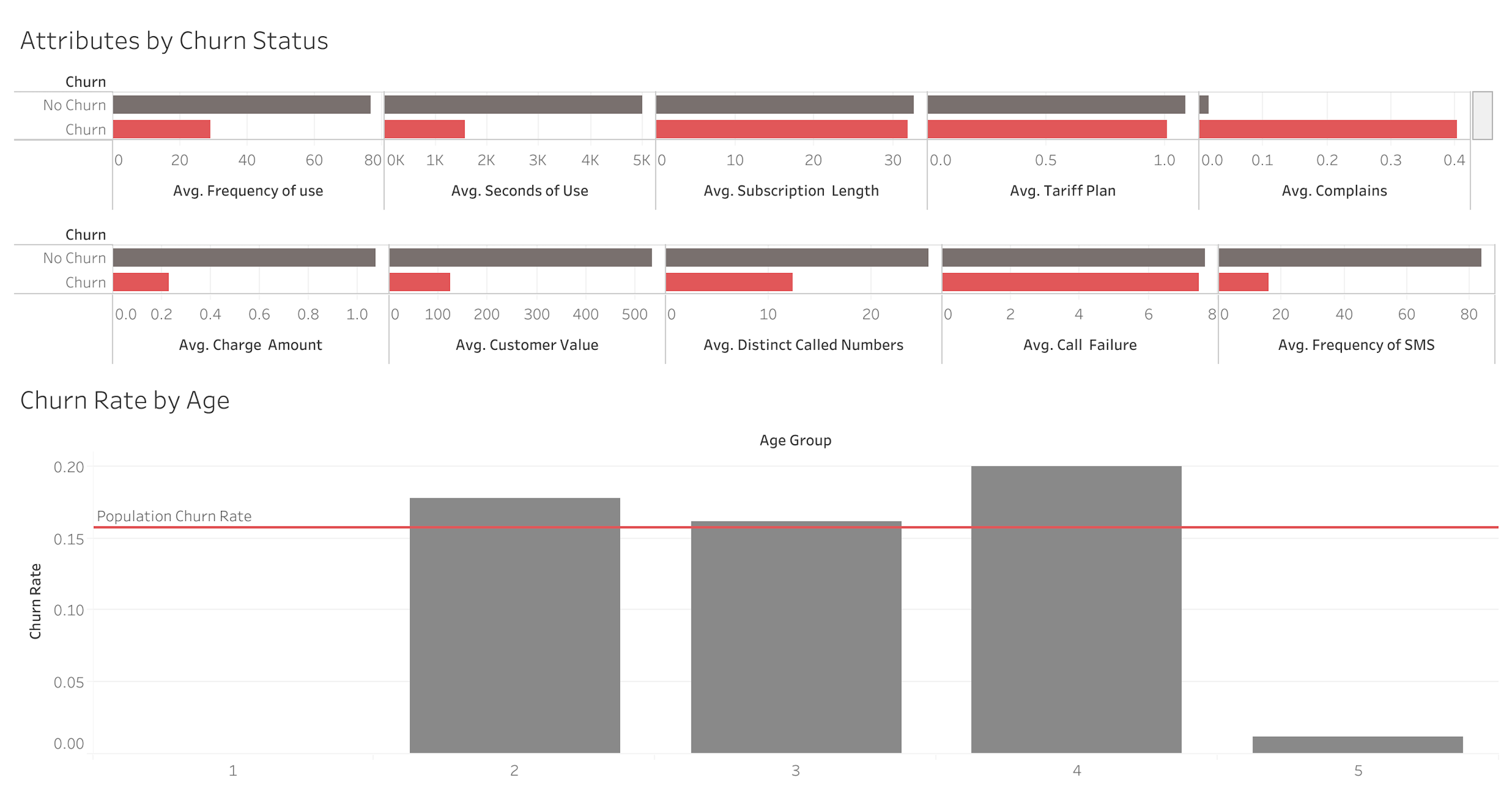
As we can see, a number of variables differ significantly between the Churn and Non-Churn group, so this dataset likely holds a good deal of useful intelligence.
正如我们所看到的,Churn和Non-Churn组之间的许多变量存在显着差异,因此此数据集可能拥有大量有用的情报。
培训和测试数据 (Training and Testing Data)
As with all Machine Learning models, we will split the data set into two parts: training and testing. We will use the training data to build the model and then evaluate the model’s performance on the test data (which the model has never seen before). We will give the model the Churn values during the training process, then, during the testing processes, we will withhold the Churn values and have the model predict them. This is how we simulate how the model would perform if deployed and used on current data to predict Churn.
与所有机器学习模型一样,我们将数据集分为两部分:训练和测试。 我们将使用训练数据来构建模型,然后根据测试数据(模型从未见过)评估模型的性能。 我们将在训练过程中为模型提供Churn值,然后在测试过程中,我们将保留Churn值并让模型进行预测。 这是我们模拟如果在当前数据上部署并使用该模型以预测客户流失时模型将如何执行的方式。
班级不平衡 (Imbalanced Classes)
The problem we are trying to solve is a Classification Problem: we are trying to take each customer and classify them into either the Non-Churn Class (denoted as a 0) or the Churn Class (denoted as a 1).
我们试图解决的问题是分类问题:我们正在尝试吸引每个客户并将其分类为非搅打类(表示为0)或搅打类(表示为1)。
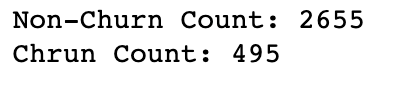
Whenever we have a classification problem, it is important to note how frequently we observe each class in the dataset. In our case, we have significantly more Non-Churn cases than we do Churn Cases, as we’d hope would be the case for any business.
每当我们遇到分类问题时,重要的是要注意我们观察数据集中每个类的频率。 在我们的案例中,与非Churn案例相比,我们的Non-Churn案例要多得多,因为我们希望任何企业都可以这样做。
Noting class imbalances is important for evaluating modeling accuracy results.
注意类不平衡对于评估建模准确性结果很重要。
For example, if I told you the model I built classifies 84% of cases correctly, that might seem pretty good. But in this case, Non-Churn cases represent 84% of the data, so, in theory, the model could just classify everything as Non-Churn and achieve an 84% accuracy score.
例如,如果我告诉您我建立的模型正确地对84%的案例进行了分类,那可能看起来还不错。 但是在这种情况下,Non-Churn案例代表了84%的数据,因此,从理论上讲,该模型可以将所有内容归类为Non-Churn,并获得84%的准确率。
Therefore, when are evaluating model performance with an imbalanced dataset, we want to judge the model based mainly on how it performs on the minority class.
因此,当使用不平衡的数据集评估模型性能时,我们要主要根据模型在少数类上的表现来判断模型。
建模结果 (Modeling Results)
As always, I will skip right to the results of the final model before diving into the modeling process, so those of you less interested in the whole process can get an understanding of the ultimate outcome and its implications.
与往常一样,在进入建模过程之前,我将直接跳至最终模型的结果,因此对整个过程不感兴趣的人可以了解最终结果及其含义。
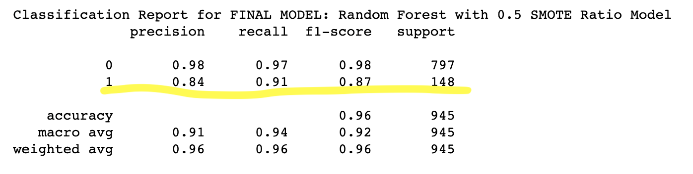
By using Synthetic Minority Over-sampling on the training data to oversample the Churn class, I was able to build a Random Forest Classifier with an overall accuracy of 96%. This means that on unseen data (test data), the model accurately predicted whether or not a customer would Churn during the next 3 months with 96% accuracy.
通过在训练数据上使用综合少数群体过度采样来对Churn类进行过度采样,我能够构建整体精度为96%的随机森林分类器。 这意味着,在看不见的数据(测试数据)上,该模型可以准确预测客户在接下来的3个月内是否会流失,准确度达到96%。
However, as we just discussed, overall accuracy does not tell the whole story!
但是,正如我们刚刚讨论的那样,整体准确性并不能说明全部问题!
Because we have imbalanced classes (84%:16%) we want to focus more on how well the model performed on the Churn cases (the minority class).
因为我们的班级不平衡(84%:16%),所以我们希望更多地关注模型在Churn案例(少数派)上的表现如何。
The below Classification Report gives us this information…
以下分类报告为我们提供了此信息…
Let’s unpack those results a little bit…
让我们对这些结果进行一些整理……
RecallA Churn class Recall of 0.91 means that the model was able to catch 91% of the actual Churn cases. This is the measure we really care about, because we want to miss as few of the true Churn cases as possible.
召回流失级别0.91意味着该模型能够捕获91%的实际流失案例。 这是我们真正关心的方法,因为我们想尽可能少地漏掉真正的Churn案例。
PrecisionPrecision of the Churn class measures how often the model catches an actual Churn case, while also factoring in how often it misclassifies a Non-Churn case as a Churn case. In this case, a Churn Precision of 0.84 is not a problem because there are no significant consequences of identifying a customer as a Churn risk when she isn’t.
精度Churn类的Precision衡量模型捕获实际Churn案例的频率,同时还考虑将模型将Non-Churn案例误分类为Churn案例的频率。 在这种情况下,客户流失精度为0.84并不是问题,因为在没有客户流失风险时将客户识别为客户流失并不会产生重大后果。
F1 ScoreThe F1 Score is the harmonic mean of Precision and Recall. It helps give us a balanced idea of how the model is performing on the Churn class. In this case a Churn Class F1 Score of 0.87 is pretty good. There is usually a trade off between Precision and Recall. I could have played around with the probability thresholds of the model and gotten Churn Class Recall up to 97%, but Churn Class Precision would have gone down since the model would be classifying a bunch of Actual Non-Churn Cases as Churn Cases. The F1 Score helps keep us honest.
F1分数F1分数是Precision和Recall的谐波平均值。 它有助于我们对模型在Churn类上的表现保持平衡。 在这种情况下,流失级F1得分为0.87是非常好的。 在Precision和Recall之间通常需要权衡取舍。 我本可以使用该模型的概率阈值,将“流失级召回率”提高到97%,但“流失级精度”将下降,因为该模型会将一堆实际的非流失案例归类为“流失案例”。 F1分数有助于保持诚实。
We can visualize this relationship with a Precision Recall Curve of the Churn Class…
我们可以通过流失级的精确召回曲线来可视化这种关系…
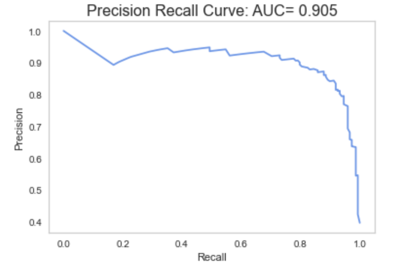
The more the curve bows out to the right, the better the model, so this model is doing well!
曲线向右弯曲的次数越多,模型越好,因此该模型运行良好!
解释最终模型 (Explaining the Final Model)
For those of you interested in what a Random Forest Classifier utilizing SMOTE means…
对于那些对使用SMOTE的随机森林分类器意味着什么感兴趣的人……
SMOTE(综合少数族裔过采样) (SMOTE (Synthetic Minority Oversampling))
SMOTE is a method for dealing with the class imbalance issue. Because our data contained only 1 Churn case for every 5.5 Churn cases, the model wasn’t seeing enough Churn cases and therefore wasn’t performing well in classifying those cases.
SMOTE是一种处理类不平衡问题的方法。 因为我们的数据中每5.5个Churn案例仅包含1个Churn案例,所以该模型没有看到足够的Churn案例,因此在对这些案例进行分类时表现不佳。
With SMOTE, we can synthesize examples of the minority class so that the classes become more balanced. Now, it is important to note that we only do this to the training data so the model can see more examples of the minority class. We do not manipulate the testing data in any way, which is what we use to evaluate the model performance.
借助SMOTE,我们可以综合少数派类别的示例,以使各个类别更加平衡。 现在,重要的是要注意,我们只对训练数据执行此操作,因此该模型可以看到少数群体的更多示例。 我们不会以任何方式操纵测试数据,这是我们用来评估模型性能的方法。
How does SMOTE create new data points out of thin air?
SMOTE如何凭空创建新的数据点?
SMOTE plots each example of the minority class in 12 Dimensional Space, since we have twelve attributes for each customer. It picks a random point from that 12D space and draws a line to that point’s nearest neighbor, then plots a new point that lies right in the middle of that line. It does this over and over again until it reaches the class ratios that you asked it for at the start.
SMOTE在12维空间中绘制少数群体类别的每个示例,因为我们为每个客户提供十二个属性。 它从该12D空间中选择一个随机点,并绘制一条与该点最近的邻居的直线,然后绘制一条恰好位于该直线中间的新点。 它会一遍又一遍地执行此操作,直到达到您在开始时要求的班级比例。
In this case, I used SMOTE on the training data to generate enough Churn class samples such that there was 1 Churn case for every 2 Non-Churn cases. This helped improve performance greatly.
在这种情况下,我在训练数据上使用了SMOTE来生成足够的Churn类样本,这样每2个Non-Churn案例中就有1个Churn案例。 这极大地提高了性能。
随机森林分类器 (Random Forest Classifier)
This is the actual model used for the Classification. A Random Forest is a collection of individual Decision Trees, and the way it works is pretty cool!
这是用于分类的实际模型。 随机森林是各个决策树的集合,其工作方式非常酷!
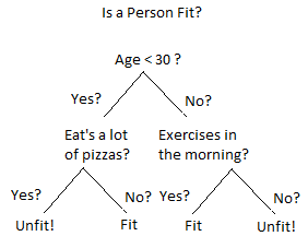
Most of us are familiar with the concept of a decision tree, even if we don’t know we are. A decision tree searches through the features available and picks the feature which, by splitting the data based on the value of that feature, will produce resulting groups that are as different from each other as possible. A picture will offer a clearer explanation…
我们大多数人都熟悉决策树的概念,即使我们不知道自己是。 决策树搜索可用的特征并选择特征,然后通过基于该特征的值拆分数据来生成结果组,这些结果组之间的差异应尽可能大。 图片将提供更清晰的解释…
A Random Forest is a collection of hundreds of different decision trees. Each individual decision tree spits out a classification, and whichever classification gets the most “votes” wins.
随机森林是数百个不同决策树的集合。 每个决策树都会列出一个类别,无论哪个类别获得最多的“票数”获胜。
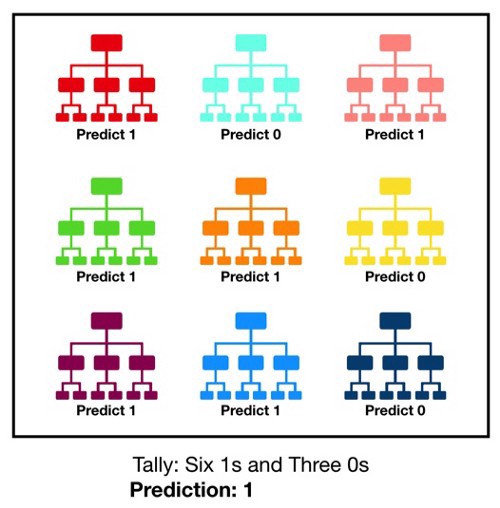
If each decision tree is splitting on the most efficient feature, then shouldn’t every decision tree in the forest be identical?The Random Forest introduces randomness in this way: every time a tree is deciding on which feature to split on, it has to chose from a random subset of features rather than the whole feature set. Thus, each individual tree in the forest is completely unique!
如果每个决策树都在最有效的功能上进行拆分,那么林中的每个决策树是否不应该完全相同? 随机森林以这种方式引入了随机性:每当一棵树决定要分割的特征时,它都必须从特征的随机子集中进行选择,而不是从整个特征集中进行选择。 因此,森林中的每一棵树都是完全独特的!
Here is the code for how to implement and evaluate a Random Forest Classifier with SMOTE…
这是有关如何使用SMOTE实施和评估随机森林分类器的代码…
# Set X to be all columns except Churn
X= df.drop(columns='Churn')
# Set y to be the Churn column
y= df['Churn'].values
# Randomly split the data into training and testing data while maintaining the same class ratios
x_train, x_test, y_train, y_test= train_test_split(X, y, test_size=0.3, stratify=y)


# create SMOTE variable with samping strat of 0.5
sm = SMOTE(sampling_strategy=0.5, random_state=12)
# apply smote to our x_train and y_train
x_train_smote, y_train_smote = sm.fit_sample(x_train, y_train)
# Check to see what the class balance looks like now
print (np.unique(y_train, return_counts=True) , np.bincount(y_train_smote))
print('\n')


# create model variables
model= RandomForestClassifier()
# fit the model on smoted trainign data
result= model.fit(x_train_smote, y_train_smote)
# make predictions
y_pred= model.predict(x_test)


# computer average score
avg_score= round(metrics.accuracy_score(y_test, y_pred),2)


# compute classification report
report= metrics.classification_report(y_test, y_pred)行动模型(The Model In Action)
Accuracy is great but how could this model be used in real life?
准确性很高,但如何在现实生活中使用该模型?
With the Random Forest model we can actually generate probabilities for each class prediction. So we can basically have the model give us a probability for each customer of how likely the model thinks that customer is to Churn over the next three months.
使用随机森林模型,我们实际上可以为每个类别预测生成概率。 因此,我们基本上可以让模型为每个客户提供一个概率,即该模型认为该客户在未来三个月内流失的可能性。
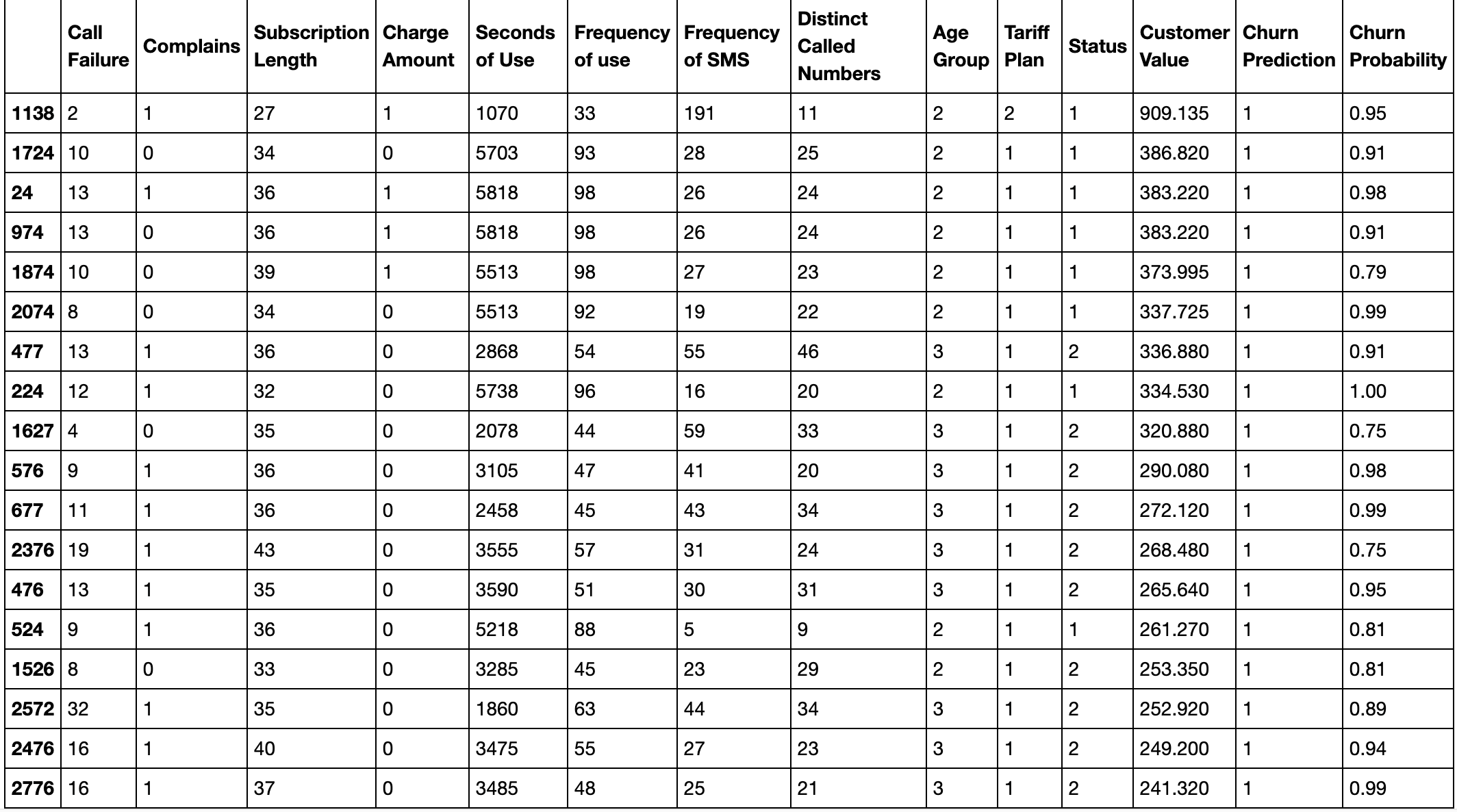
For example, we could return a list of all customers who have a greater than 65% chance of Churning. Since we really only care about high value customers, we could make it so that list contains only those customers with a higher than average Customer Value.
例如,我们可以返回所有有超过65%机会进行搅动的客户的列表。 由于我们实际上只关心高价值的客户,因此我们可以做到这一点,以便该列表仅包含那些具有高于平均客户价值的客户。
In doing so, we are able to generate a list of customers who are of high value to the company and are at high risk of Churning. These are the customers with which the company would want to intervene in some way to get them to stay.
这样一来,我们便能够生成对公司具有高价值并有高搅动风险的客户清单。 这些客户是公司希望以某种方式进行干预以使其停留的客户。
When run on testing data, such a list looks like this (the index is the Customer ID)…
在测试数据上运行时,这样的列表看起来像这样(索引是客户ID)…
Here is the code for generating such a list after fitting the model like we did above…
这是在像我们上面所做的那样拟合模型之后生成此类列表的代码…
# Predict the probabilities from model and covert to a list
proba= result.predict_proba(x_test)
proba_list=proba.tolist()


# The probability of churn is the second value in each nested list so we want to loop through and pull that
# value out into it's own list
churn_prob=[]
for item in proba_list:
    churn_prob.append(item[1])


# create a df that is copy of x_test
df_prob= x_test.copy()


# add our churn prediction and the subsequent probability of churn to the df
df_prob['Churn Prediction']= y_pred
df_prob['Churn Probability']= churn_prob


# Etablish a reference point for above average value customers
median_value= df_prob['Customer Value'].median()
# Establish a point for what it means to be at high risk of churning
high_prob= 0.65


# Create a df of just those who are of above avergae value and are at high risk of churning
high_risk_df= df_prob[(df_prob['Customer Value'] >= median_value) & (df_prob['Churn Probability'] > high_prob)].sort_values(by='Customer Value', ascending=False)
# View the list
print(high_risk_df)了解每个功能如何促成客户流失(Understanding How Each Feature Contributes to Churn)
Being able to predict those customers who are likely to Churn is great, but, if this were my company I’d also want to know how each feature is contributing to Churn.
能够预测可能会造成客户流失的客户很棒,但是,如果这是我的公司,我还想知道每个功能如何为客户流失做出贡献。
Just by visualizing the data like we did in the Visualizing the Data section, we could see how each individual features relates to Churn. Unfortunately, it’s tough to compare the effect of each variable based solely on visualization.
就像我们在“可视化数据”部分中所做的那样,通过可视化数据,我们可以看到每个单独的功能如何与客户流失相关。 不幸的是,很难仅基于可视化来比较每个变量的效果。
We can actually use another Machine Learning technique, called Logistic Regression, to compare the effects of each feature. Logistic Regression is also a classification model. In our case, it didn’t give us prediction performance that was as good as Random Forest, but it does give us good, interpretable information on how each feature affects Churn.
实际上,我们可以使用另一种称为Logistic回归的机器学习技术来比较每个功能的效果。 Logistic回归也是一种分类模型。 在我们的案例中,它的预测性能不如“随机森林”那么好,但确实为我们提供了有关每个要素如何影响用户流失率的良好且可解释的信息。
The Logistic Regression Coefficients are visualized below…
Logistic回归系数如下图所示:
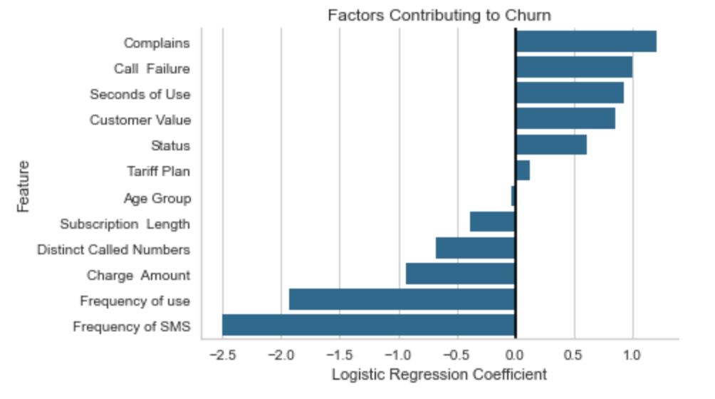
Features with positive coefficients mean that an increase in that feature leads to an increased chance in that observation being a Churn case.
具有正系数的特征意味着该特征的增加导致该观察为Churn案例的机会增加。
Features with negative coefficients mean that an increase in that feature leads to a decreased chance in that observation being a Churn case.
具有负系数的特征意味着该特征的增加导致该观察为Churn案例的机会减少。
So the more Call Failures recorded for a customer, the more likely that customer is to be a Churn case. The more SMS messages sent by a customer (‘Frequency of SMS’), the less likely that customer is to be a Churn case.
因此,为客户记录的呼叫失败次数越多,该客户成为客户流失案例的可能性就越大。 客户发送的SMS消息越多(“ SMS频率”),则客户成为流失案例的可能性就越小。
Here is the code for computing and plotting those coefficients…
这是用于计算和绘制这些系数的代码……
# establish model
model= LogisticRegression()
# fit model on scaled and smoted data
result= model.fit(x_train_scaled_smote, y_train_smote)
# make predictions
y_pred= model.predict(x_test_scaled)


# get the coefficnt values
coefficients= result.coef_.tolist()[0]
# get the feature names
features= list(x_train.columns)


# Add features and their importance to the dataframe
logit_df['Feature']= features
logit_df['Coefficient']= coefficients


# Sort the dataframe by coefficient value
logit_df= logit_df.sort_values(by='Coefficient', ascending=False )


# plot the dataframe
sns.barplot(x='Coefficient', y= 'Feature', data=logit_df, color='b')
plt.title('Factors Contributing to Churn')
plt.xlabel('Logistic Regression Coefficient')
plt.axvline(x=0, color='black')
sns.despine()建模迭代(Modeling Iterations)
As always, I tried multiple different models and over sampling techniques before settling on Random Forest with SMOTE.
与往常一样,在使用SMOTE适应Random Forest之前,我尝试了多种不同的模型和过采样技术。
Models Tried:- Logistic Regression-Random Forest-Gradient Boosting Classifier-Ada Boost Classifier
尝试过的模型:-Logistic回归-随机森林梯度提升分类器-Ada Boost分类器
Oversampling Techniques Tried:-No oversampling (imbalanced classes)-SMOTE w/ 0.25, 0.5,0.75 and 1 as class ratios-ADASYN w/ 0.25, 0.5, 0.75 and 1 class ratios
尝试过采样技术:-无过采样(不平衡类)-SMOTE w / 0.25、0.5、0.75和1类比-ADASYN w / 0.25、0.5、0.75和1类比
To compare the models, I tried each model with each sampling strategy. I added all results to a dataframe that looked like this…
为了比较模型,我尝试了每种模型和每种抽样策略。 我将所有结果添加到如下所示的数据框中…
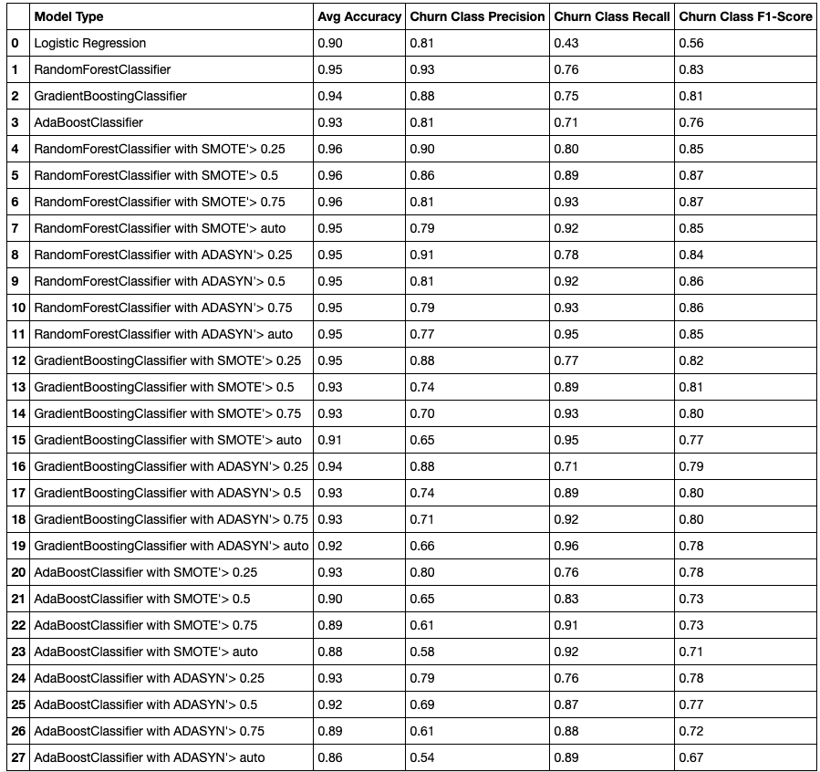
This dataframe was put together with the following two code blocks (except for Logistic Regression models, which had to be computed separately due to the need to scale the X variables)…
该数据帧与以下两个代码块放在一起(除了Logistic回归模型外,由于需要缩放X变量,因此必须分别计算该模型)…
# establish list of models
models= [RandomForestClassifier(), GradientBoostingClassifier(), AdaBoostClassifier()]


# Loop through model types and build a model for each model type while adding performance metrics to model_performance df
for model in models:
    model_name= str(model)[:-2]
    # create model variables
    model= model
    # fit the model
    result= model.fit(x_train, y_train)
    # make predictions
    y_pred= model.predict(x_test)


    # computer average score
    avg_score= round(metrics.accuracy_score(y_test, y_pred),2)


    # compute classification report
    report= metrics.classification_report(y_test, y_pred)
    print('Classification Report for {} Model'.format(model_name))
    print(report)


    # get classification report as dict
    report_dict= metrics.classification_report(y_test, y_pred, output_dict=True)
    # get only metrics for churn class
    report_churn= list(report_dict['1'].values())
    # pull out individual churn metrics
    churn_precision= round(report_churn[0],2)
    churn_recall= round(report_churn[1], 2)
    churn_f1= round(report_churn[2], 2)


    # add model metrics to the data frame
    new_row={'Model Type': model_name, 'Avg Accuracy': avg_score, 'Churn Class Precision': churn_precision,
             'Churn Class Recall': churn_recall, 'Churn Class F1-Score': churn_f1}
    model_performance= model_performance.append(new_row, ignore_index=True)

 # create list of different sampling strategies
ratios= [0.25, 0.5, 0.75, 'auto']
# create list of oversampling techiques
oversample_techniques= [SMOTE, ADASYN]


# Loop through model types
for model in models:
    # For each model type build a model using each over sampling technique
    for technique in oversample_techniques:
        # for each over sampling technique build a model using each different sampling ratio
        for ratio in ratios:
            model_name= '{} with {} {}'.format(str(model)[:-2], str(technique).split('.')[3], ratio)
            sample_method= technique(sampling_strategy=ratio)
            x_train_smote, y_train_smote= sample_method.fit_sample(x_train, y_train)
            # establish model
            model= model
            # fit model
            result= model.fit(x_train_smote, y_train_smote)
            # make predictions
            y_pred= model.predict(x_test)


            # computer average score
            avg_score= round(metrics.accuracy_score(y_test, y_pred),2)


            # compute classification report
            report= metrics.classification_report(y_test, y_pred)
            print('Classification Report for {} Model'.format(model_name))
            print(report)


            # get classification report as dict
            report_dict= metrics.classification_report(y_test, y_pred, output_dict=True)
            # get only metrics for churn class
            report_churn= list(report_dict['1'].values())
            # pull out individual churn metrics
            churn_precision= round(report_churn[0],2)
            churn_recall= round(report_churn[1], 2)
            churn_f1= round(report_churn[2], 2)


            # add model metrics to the data frame
            new_row={'Model Type': model_name, 'Avg Accuracy': avg_score, 'Churn Class Precision': churn_precision,
                     'Churn Class Recall': churn_recall, 'Churn Class F1-Score': churn_f1}
            model_performance= model_performance.append(new_row, ignore_index=True)
So that is how you can use Machine Learning to predict and prevent the Churn of High Value Customers. To recap, we were able to accomplish two major things using machine learning that we couldn’t have done with “traditional” visualization based analytics. We were able to:1) Generate a model that can identify 90% of Churn cases before they happen2) Rank order how each factor contributes to the probability of a customer Churning.
这样便可以使用机器学习来预测和防止高价值客户流失。 概括地说,我们能够使用机器学习完成两项主要工作,而这是基于“传统”可视化的分析无法做到的。 我们能够:1)生成一个模型,该模型可以在90%的客户流失案例发生之前对其进行识别。2)对每个因素如何影响客户流失的可能性进行排序。
谢谢阅读!! (Thanks for Reading!!)
机器学习 客户流失


 281
281


 被折叠的 条评论
为什么被折叠?
被折叠的 条评论
为什么被折叠?
 到【灌水乐园】发言


