pca 主成分分析_vc pca主成分分析

最新推荐文章于 2021-10-12 13:50:40 发布

weixin_26713457

最新推荐文章于 2021-10-12 13:50:40 发布

阅读量193

点赞数

原文链接：https://medium.com/swlh/vc-pca-principal-component-analysis-a4f02ba719c5

版权

pca 主成分分析

I explained about how we visualize high dimensional data in the 2D graph. It was not about the dimensionality reduction. This post and the following posts will explain how we embed high-dimensional data into a low dimensional space. I will explain PCA, Kernel PCA, MDS, ISOMAP, and t-SNE. This post will show you all about PCA and Kernel PCA.

我解释了如何在2D图形中可视化高维数据。这与降维无关。这篇文章和后面的文章将解释我们如何将高维数据嵌入到低维空间中。我将解释PCA，内核PCA，MDS，ISOMAP和t-SNE。这篇文章将向您展示有关PCA和内核PCA的所有信息。

PCA (PCA)

Basically, PCA is trying to find the best basis. It is orthogonal to each other and the best representative based on its variation. The distance from the PCA basis to original data points is minimized and the next PCA basis will not take into account the previous variation, this point makes the orthogonal basis. This is the basic intuition of PCA.

基本上，PCA试图寻找最佳基础。它彼此正交，并且是基于其变化的最佳代表。从PCA基础到原始数据点的距离最小，下一个PCA基础将不考虑先前的变化，该点构成正交基础。这是PCA的基本直觉。

Goals of Principal Component Analysis

主成分分析的目标

Image for post — Centered x is mapping into y by matrix U

First of all, we need to standardize the original data because it's the absolute data size affects the result of PCA. Changing the basis is just mapping in linear algebra language. U in the equation is what we are trying to find in order to change the basis. The condition of U is to minimize the approximated error. In this way, the variance in the projected data remains maximal because we project x onto the basis keeping the variance. However, it has a limitation the PCA only considers the linear relationship. I will elaborate on these steps.

首先，我们需要对原始数据进行标准化，因为它的绝对数据大小会影响PCA的结果。改变基础只是线性代数语言中的映射。等式中的U是我们试图找到的以更改基数。 U的条件是使近似误差最小。这样，由于我们将x投影到保持方差的基础上，所以投影数据中的方差保持最大。但是，PCA仅考虑线性关系具有局限性。我将详细说明这些步骤。

Setting the origin of the new axes

设置新轴的原点

We need to find the center to standardize the origin data. In PCA, it will be the mean of the original data because it has the minimum sum of the distance between all data points.

我们需要找到中心来标准化原点数据。在PCA中，它是原始数据的均值，因为它具有所有数据点之间的最小距离之和。

The variance of projected points

投影点的方差

We define the line through the center of mass m and project original points x onto it. The sample variance of the projected points x’ is maximized and selects the line as a principal component. We can calculate the variance more easily with simple linear algebra because the variance actually is dot products.

我们定义了一条穿过质心m的线，并将原始点x投射到其上。投影点x'的样本方差最大化，并选择该线作为主要成分。我们可以使用简单的线性代数更轻松地计算方差，因为方差实际上是点积。

The above picture tells the whole process of projection and how to find the variation. Now, we are going to calculate this with linear algebra.

上图说明了投影的整个过程以及如何找到变化。现在，我们将使用线性代数进行计算。

线性代数计算 (Linear Algebra Calculation)

This part will explain how we calculate the U (the matrix map the original data on PCA basis.)with linear algebra.

本部分将说明我们如何使用线性代数计算U(矩阵以PCA为基础映射原始数据)。

Scatter Matrix

散点矩阵

First of all, we need to define our scatter matrix. This is true by its definition and you can understand this is the symmetric matrix, it has all real eigenvalue and its eigenvectors are orthogonal. We can show the scatter matrix S determines the sample variance in direction v:

首先，我们需要定义分散矩阵。根据其定义，这是正确的，您可以理解这是对称矩阵，它具有所有实特征值，并且其特征向量是正交的。我们可以显示出散射矩阵S确定了方向v上的样本方差：

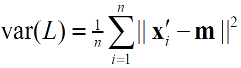
We change vectors to the matrix and power to dot product. According to the Min-Max theorem of linear algebra, the extrema of var(L) are attained at the eigenvectors of S because vector v length is 1. Finally, we can calculate the maximal and minimal variance by eigenvalue decomposition of s. As I mentioned above, the S is a symmetric matrix.

我们将向量更改为矩阵，并乘以点积。根据线性代数的最小-最大定理，由于向量v的长度为1，因此在S的特征向量处获得var(L)的极值。最后，我们可以通过s的特征值分解来计算最大和最小方差。如上所述，S是一个对称矩阵。

Now, we got U it is from eigenvectors of scatter matrix surprisingly and each eigenvector is connected to each eigenvector sorted by descending order(lambda 1 is the biggest one, therefore it contains the biggest variance.). If you want to check the relationship between PCA and SVD with this point. Please take a look at this lecture:

现在，我们惊奇地从散布矩阵的特征向量中得到了U，每个特征向量都与按降序排序的每个特征向量相连(λ1是最大的，因此包含最大的方差)。如果要检查PCA和SVD之间的关系，请注意这一点。请看一下这堂课：

演示地址

The SVD and PCA

SVD和PCA

Algorithm for PCA

PCA算法

Input: the data, p-dimensional spaceOutput: the embedded data by Uk. U is selected by k, it determines how many columns we choose for the result.

输入：数据，p维空间输出：Uk嵌入的数据。 U由k选择，它确定我们为结果选择多少列。

Process:1. Center the points with mean: X - mean of X2. Define the scatter matrix S by centered X3. Compute the eigendecomposition and get U.4. Define Uk by given k.

Craft.io：1。用均值将点居中：X-X2的均值。通过居中X3定义散射矩阵S。计算特征分解并得到U.4。用给定的k定义Uk。

In the next post, I will explain how to solve the limitation of PCA, only represent the linear relationship, by kernel trick.

在下一篇文章中，我将通过内核技巧来说明如何解决PCA的局限性，仅代表线性关系。

This post is published on 9/4/2020.

此帖发布于9/4/2020。