神经网络 深 浅_神经网络为什么更深的总不总是更好

神经网络 深 浅

When creating Neural Networks, one has to ask: how many hidden layers, and how many neurons in each layer are necessary?

创建神经网络时，必须问：隐藏的层数以及每层中需要多少个神经元？

When it comes to complex real data, Andrew Ng suggests in his course on Coursera: Improving Deep Neural Networks, that it is a highly iterative process, and so we have to run many tests to find the optimal hyperparameters.

当涉及到复杂的真实数据时，Andrew Ng在他的Coursera课程：改进深度神经网络中建议，这是一个高度迭代的过程，因此我们必须运行许多测试才能找到最佳的超参数。

But, what is the intuition behind how the hidden layers and neurons impact the final model?

但是，隐藏层和神经元如何影响最终模型的直觉是什么？

简单的非线性可分离数据 (Simple non-linearly separable data)

Let’s create a dataset using make_circles.

让我们使用make_circles创建一个数据集。

from sklearn import datasetsX,y=datasets.make_circles(n_samples=200,shuffle=True, noise=0.1,random_state=None, factor=0.1)

And you can visualize the dataset:

您可以可视化数据集：

import matplotlib.pyplot as plt
plt.scatter(X[:, 0], X[:, 1], c=y,s=20)
plt.axis(‘equal’)

Image by Author

图片作者

神经元和层如何？(How may neurons and layers?)

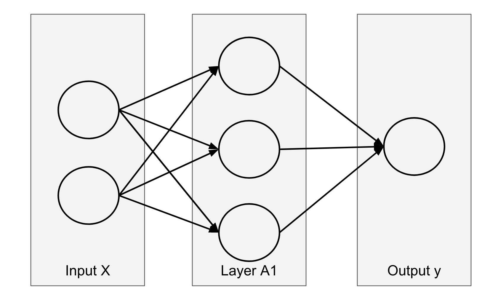
Each neuron creates a linear decision boundary. By looking at the dataset, the intuition is to create one layer of 3 neurons. And we should be able to create a perfect classifier. Now, what about only 2 neurons? It seems not enough, and what if we try to add more layers?

每个神经元创建一个线性决策边界。 通过查看数据集，直觉是创建3个神经元的一层。 而且我们应该能够创建一个完美的分类器。 现在，只有2个神经元呢？ 似乎还不够，如果我们尝试添加更多的层怎么办？

With these questions, let’s try to do some tests.

带着这些问题，让我们尝试做一些测试。

一层隐藏层中有3个神经元 (3 neurons in one hidden layer)

If we use 3 neurons with the following code:

如果我们用以下代码使用3个神经元：

from sklearn.neural_network import MLPClassifierclf =MLPClassifier(solver=’lbfgs’,hidden_layer_sizes(3,),
activation=”tanh”,max_iter=1000)clf.fit(X, y)
clf.score(X,y)

Then we are able to create 3 decision boundaries within the hidden layer. And we can notice that there are an infinite number of possibilities to create these 3 lines (so there are an infinite number of global minimum in the cost function of this neural network).

然后，我们可以在隐藏层中创建3个决策边界。 我们可以注意到，创建这3条线的可能性是无限的(因此，该神经网络的成本函数中的全局最小值有无限的可能性)。

Image by Author

图片作者

To create the visualization of the decision boundaries of the hidden layer, we can use the coefficients and intercepts of the hidden layer.

为了创建隐藏层决策边界的可视化，我们可以使用隐藏层的系数和截距。

n_neurons=3xdecseq=np.repeat(np.linspace(-1,1,100),n_neurons).reshape(-1,n_neurons)ydecseq=-(xdecseq*clf.coefs_[0][0]+clf.intercepts_[0])/clf.coefs_[0][1]

Then we can plot these three lines with the original dataset:

然后，我们可以用原始数据集绘制这三条线：

fig, ax = plt.subplots(figsize=(8,8))ax.scatter(X[:, 0], X[:, 1], c=y,s=20)ax.plot(xdecseq[:, 0], ydecseq[:, 0])
ax.plot(xdecseq[:, 1], ydecseq[:, 1])
ax.plot(xdecseq[:, 2], ydecseq[:, 2])ax.set_xlim(-1.5, 1.5)
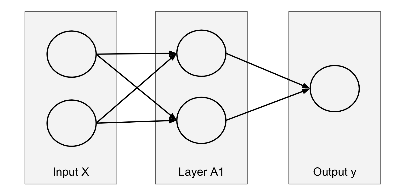
ax.set_ylim(-1.5, 1.5)

一个隐藏层中2个神经元 (2 neurons in one hidden layer)

If we use only 2 neurons, it is quite easy to see that we will not be able to perfectly classify all observations.

如果仅使用2个神经元，则很容易看出我们将无法对所有观察结果进行完美分类。

Using similar codes, we can plot the following graph with 2 decision boundaries from the hidden layer.

使用类似的代码，我们可以从隐藏层绘制具有2个决策边界的下图。

Image by Author

图片作者

2个神经元，每个神经元有很多层(2 neurons each with many layers)

What if we create 2 neurons in many hidden layers? To better understand what happened in the first hidden layer with 2 neurons, I created this visualization.

如果我们在许多隐藏层中创建2个神经元怎么办？ 为了更好地了解具有2个神经元的第一个隐藏层中发生的情况，我创建了此可视化。

Image by Author

图片作者

Now it is quite clearly that no matter how many layers you add, you will never to able to classify the data in the red circle below.

现在很明显，无论您添加多少层，都将永远无法在下面的红色圆圈中对数据进行分类。

Image by Author

图片作者

You can test yourself: you can add more layers in the argument hidden_layer_sizes. For example (2,3,2) means 3 hidden layers with 2, 3, and 2 neurons for each.

您可以测试自己：您可以在参数hidden_​​layer_sizes中添加更多层。 例如(2,3,2)表示3个隐藏层，每个都有2、3和2个神经元。

from sklearn.neural_network import MLPClassifierclf = MLPClassifier(solver=’lbfgs’,
hidden_layer_sizes=(2,3,2),
activation=”tanh”,max_iter=1000)clf.fit(X, y)
clf.score(X,y)

结论 (Conclusions)

From this simple example, we can end with this intuition:

从这个简单的例子，我们可以得出以下直觉：

• The number of neurons in the first hidden layer creates as many linear decision boundaries to classify the original data.
  第一隐藏层中神经元的数量创建了尽可能多的线性决策边界以对原始数据进行分类。
• It is not helpful (in theory) to create a deeper neural network if the first layer doesn’t contain the necessary number of neurons.
  如果第一层不包含必要数量的神经元，则在理论上创建更深的神经网络是没有帮助的。

If you want to see other animations to understand how neural networks work, you can also read this article.

如果要查看其他动画以了解神经网络的工作原理，也可以阅读本文。

翻译自: https://towardsdatascience.com/neural-network-why-deeper-isnt-always-better-2f862f40e2c4

神经网络 深 浅