automl_automl diy版

automl

Written by Eric He, Nafis Asghari, Max Howarth and Colin Roos — July 7th, 2020

由 Eric He ， Nafis Asghari ， Max Howarth 和 Colin Roos 撰写 -2020年7月7日

Automated machine learning is making leaps and bounds. Gone are the days where you need a master’s degree in math to build yourself an efficient neural network.

自动化机器学习正在突飞猛进。 需要一个数学硕士学位来建立一个高效的神经网络的日子已经一去不复返了。

Tools such as Google’s AutoML Vision, Auto-PyTorch, and Auto-Keras have made some significant progress in the Neural Architecture Search (NAS) space. Additionally, we no longer need to do exhaustive grid searches to yield a highly-tuned model.

Google的AutoML Vision，Auto-PyTorch和Auto-Keras等工具在神经体系结构搜索(NAS)领域取得了重大进展。 此外，我们不再需要进行详尽的网格搜索来生成高度调整的模型。

Automated machine learning does not come cheap, though; it is often computationally expensive to test a growing search space. Enormous compute capacity is one advantage of Google’s AutoML tools. However, heavy computing loads can be migrated to run in a cloud environment to replicate the ability of AutoML.

但是，自动化机器学习并不便宜。 测试不断增长的搜索空间在计算上通常很昂贵。 巨大的计算能力是Google AutoML工具的优势之一。 但是，可以将繁重的计算负载迁移到云环境中运行，以复制AutoML的功能。

This tutorial will teach you how to allocate a virtual machine on Google’s Cloud Platform, set it up to run Auto-Keras and search for an optimized model, and deploy your model using an API for production use.

本教程将教您如何在Google的Cloud Platform上分配虚拟机，如何将其设置为运行Auto-Keras并搜索优化的模型，以及如何使用用于生产的API部署模型。

第1部分：走向云，我们开始！ (Part 1: To The Cloud, We Go!)

If you don’t already have a Google Cloud account, you can create a free one and get some credits while you’re at it. Use the link below to sign up for the free trial.

如果您还没有Google Cloud帐户，则可以创建一个免费帐户，并获得一些积分。 使用下面的链接注册免费试用。

Once you set up your account, go to console.cloud.google.com to get started setting up a VM. You should see something like the screenshot below.

设置帐户后，请转到console.cloud.google.com开始设置虚拟机。 您应该会看到类似下面的屏幕快照。

The GCP Dashboard, you should land here. GCP信息中心，您应该在这里着陆。

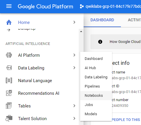
Click the Navigation Menu using the hamburger in the top left corner. Scroll down to the Artificial Intelligence section and select AI Platform > Notebooks.

使用左上角的汉堡包单击导航菜单。 向下滚动到“ 人工智能”部分，然后选择“ AI平台”>“笔记本” 。

Launch the AI Platform Notebooks Dashboard.

启动AI平台笔记本仪表板。

Create a new Notebook instance using the Create Instance button at the top of the screen. You will need to select the CUDA Toolkit 10.1 without GPU.

使用屏幕顶部的“创建实例”按钮创建一个新的Notebook实例。 您将需要选择不带GPU的CUDA Toolkit 10.1 。

Creating a new AI Notebooks VM Instance.

创建一个新的AI Notebooks VM实例。

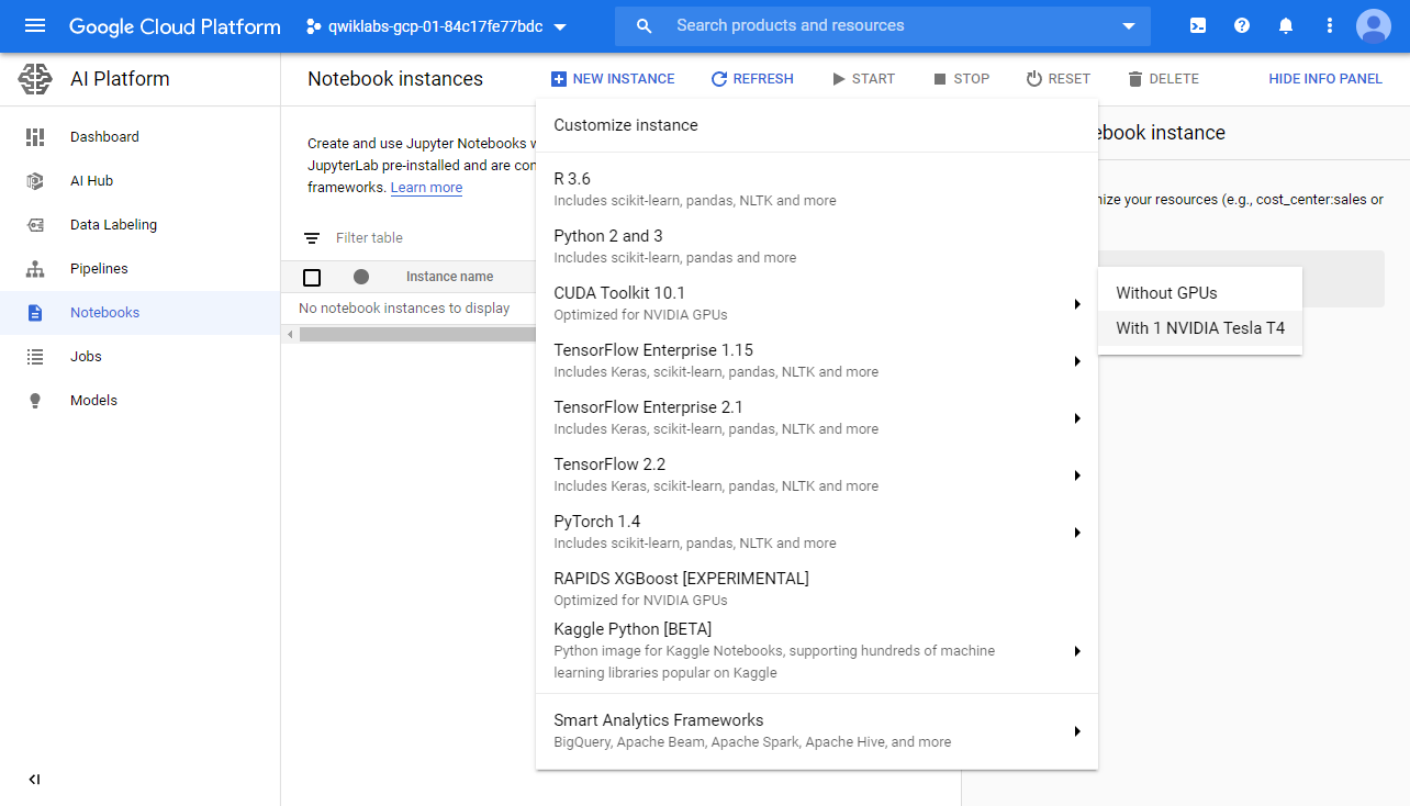
Note — Follow the optional steps below to configure GPU compute, there are a few more hoops to jump through.

注意—请按照以下 可选步骤 配置GPU计算，还有更多困难需要克服。

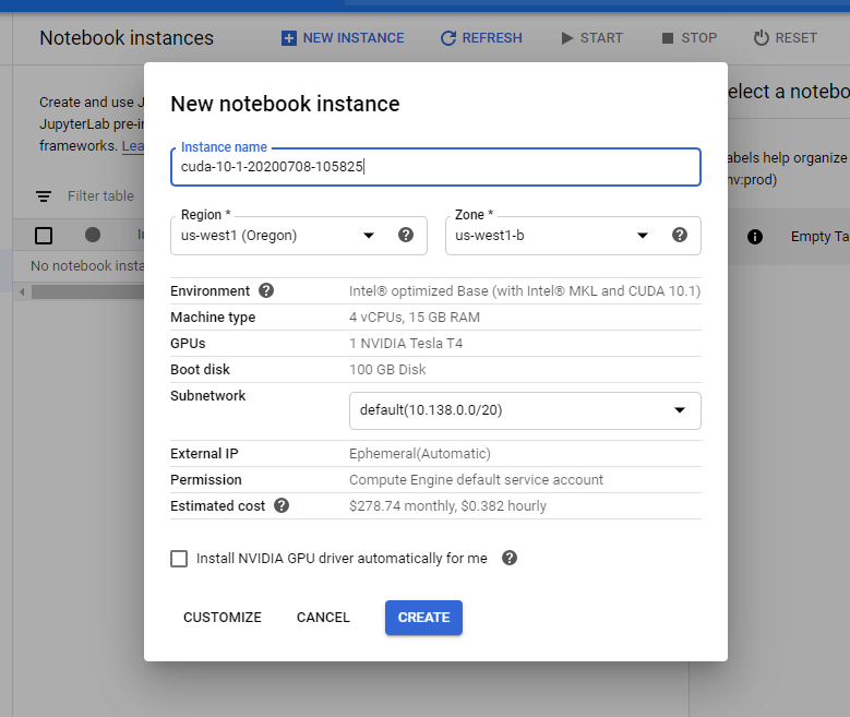
Selecting this option will bring you to a pop-up to configure the VM instance. The default name is fine unless you have a specific one in mind. VM Instance names must be globally unique.

选择此选项将带您弹出配置VM实例的窗口。 除非您有特定的名称，否则默认名称很好。 VM实例名称必须是全局唯一的。

It’s best to choose a region and zone that is closest to your physical location, but not all regions will have the infrastructure available to fulfill the instance request. You may have to try a few zones if you are having trouble getting the instance allocated.

最好选择最接近您的物理位置的区域和区域，但是并非所有区域都具有可用于满足实例请求的基础结构。 如果无法分配实例，则可能必须尝试几个区域。

Region and 区域和 Zone that makes sense for your location. 区域” 。

It will take a few minutes for the VM to be allocated and start. Once it is finished, it will look something like this:

分配和启动虚拟机需要几分钟。 完成后，它将类似于以下内容：

Wait for the VM to be allocated, you will get a green checkmark when it’s up and running.

等待分配虚拟机，启动并运行时，您会看到一个绿色的选中标记。

Click the OPEN JUPYTERLAB button to launch a new window with JupyterLab running on the VM.

单击OPEN JUPYTERLAB按钮以在VM上运行JupyterLab的情况下启动新窗口。

Open a terminal window and install some packages.

打开终端窗口并安装一些软件包。

Click on Terminal under the Other subsection of the Launcher.

单击启动器“ 其他”子部分下的“ 终端 ”。

Run the command:

运行命令：

pip install autokeras
pip install tensorflow-datasets

Wait for Auto-Keras and its dependencies to install.

等待Auto-Keras及其依赖项安装。

The kerastuner package must be manually installed in addition to Auto-Keras.

除Auto-Keras外，还必须手动安装kerastuner软件包。

Run the command:

运行命令：

pip install git+https://github.com/keras-team/keras-tuner.git@b9f314cde07ec6d54fdf5c7db1cd8f2c76ac53e6

This command clones a git repository and installs the package directly from a repository hosted on GitHub instead of the usual pypi.org.

此命令克隆git存储库，并直接从GitHub托管的存储库而不是通常的pypi.org安装软件包。

Wait for kerastuner to finish installing.

等待kerastuner完成安装。

Go to file> New > Notebook to create a new Jupyter Notebook.

转到文件>新建>笔记本以创建新的Jupyter笔记本。

Create a new Jupyter Notebook.

创建一个新的Jupyter Notebook。

Now we’re ready to write some code!

现在我们准备编写一些代码！

第2部分：编写一些代码 (Part 2: Writing Some Code)

Now that you’ve got the VM environment setup and a new notebook running, let’s put together a few lines of code to do a model architecture search that best fits the Tensorflow Rock-Paper-Scissors dataset.

既然您已经设置了VM环境并正在运行一个新的Notebook，那么我们将几行代码放在一起，以进行最适合Tensorflow Rock-Paper-Scissors数据集的模型体系结构搜索。

We need to import a few libraries to get started:

我们需要导入一些库以开始使用：

import autokeras as ak
import tensorflow_datasets as tfds

We also need to do a bit of data wrangling to get the dataset ready to training:

我们还需要做一些数据整理以使数据集准备好进行训练：

# Training Data
ds_train = tfds.load('RockPaperScissors', 
                     split='train', 
                     shuffle_files=True, 
                     batch_size = -1)


# Convert the Dataset to a numpy object
ds_numpy = tfds.as_numpy(ds_train)


# Extract the image and label
X_train, y_train = ds_numpy["image"], ds_numpy["label"]


# Check the dimensions
print(X_train.shape)  # (2520, 300, 300, 3)
print(y_train.shape)  # (2520,)


# Testing Data
ds_test = tfds.load('RockPaperScissors', 
                    split='test', 
                    shuffle_files=False, 
                    batch_size = -1)
ds_numpy = tfds.as_numpy(ds_test)


X_test, y_test = ds_numpy["image"], ds_numpy["label"]

Auto-Keras has a straightforward API, and as such, the modelling portion boils down to the following lines of code:

Auto-Keras具有直接的API，因此，建模部分可归结为以下代码行：

classifier = ak.ImageClassifier(max_trials=1)
classifier.fit(X_train, y_train, epochs=5)

Note — We recommend only setting 1 trial, this will still search long enough for you to enjoy a beer. If you want to search some more, we strongly recommend following the instructions below to allocate a GPU resource.

注意—我们建议仅设置1次试用，这仍然会搜索足够长的时间，以供您品尝啤酒。 如果您想搜索更多内容，我们强烈建议您按照以下 说明 分配GPU资源。

These two simple lines of code will find the best model for your dataset using a fancy neural architecture search method. You can read more about how this works in the original Auto-Keras paper.

这两条简单的代码行将使用一种花哨的神经体系结构搜索方法为您的数据集找到最佳模型。 您可以在原始Auto-Keras论文中阅读有关此工作原理的更多信息。

Auto-Keras will print the trial configuration to the terminal whenever it completes a trial. It gives you the score it gave that model along with the hyperparameters for that specific model trial. You can see here that it used a straightforward model with a vanilla convolutional block.

每当Auto-Keras完成试用时，它将在终端上打印试用配置。 它为您提供了该模型的得分以及该特定模型试验的超参数。 您可以在这里看到它使用了带有卷积块的简单模型。

[Trial complete]
[Trial summary]
  |-Trial ID: 4a91941f4f26fea619c06f2231924400
  |-Score: 0.04680884629487991
  |-Best step: 2
  > Hyperparameters:
  |-classification_head_1/dropout_rate: 0.5
  |-classification_head_1/spatial_reduction_1/reduction_type:   flatten
  |-image_block_1/augment: False
  |-image_block_1/block_type: vanilla
  |-image_block_1/conv_block_1/dropout_rate: 0.25
  |-image_block_1/conv_block_1/filters_0_0: 32
  |-image_block_1/conv_block_1/filters_0_1: 64
  |-image_block_1/conv_block_1/kernel_size: 3
  |-image_block_1/conv_block_1/max_pooling: True
  |-image_block_1/conv_block_1/num_blocks: 1
  |-image_block_1/conv_block_1/num_layers: 2
  |-image_block_1/conv_block_1/separable: False
  |-image_block_1/normalize: True
  |-optimizer: adam

We can also evaluate the model on the test subset using some metric functions from the scikit-learn package. Note that we need to specify a micro-averaging for the F1 scoring function because of the multi-class labels.

我们还可以使用scikit-learn包中的某些指标函数在测试子集上评估模型。 请注意，由于有多个类别的标签，我们需要为F1评分功能指定微平均值。

from sklearn.metrics import f1_score, accuracy_scorey_pred = classifier.predict(X_test)f1 = f1_score(y_test, y_pred, average=’micro’)
accuracy = accuracy_score(y_test, y_pred)print(f'F1: {f1:.3f}    Accuracy: {accuracy:.3f}')>>> F1: 0.975    Accuracy: 0.975

The best model can be saved by first exporting it and then saving it like any other Tensorflow model.

可以先导出最佳模型，然后再像其他任何Tensorflow模型一样保存它，以保存最佳模型。

best_model = classifier.export_model()try:
  best_model.save('./best_model', save_format='tf')
except:
  best_model.save('./best_model.h5')

自定义搜索空间 (Custom Search Space)

We can also define a custom search space, primarily looking for the best hyperparameters instead of the architecture. Here, we will build the following model:

我们还可以定义一个自定义搜索空间，主要是寻找最佳的超参数而不是架构。 在这里，我们将构建以下模型：

A simple image classifier search space.

一个简单的图像分类器搜索空间。

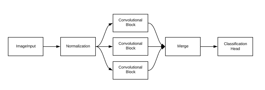
input_node = ak.ImageInput()
output_node = ak.Normalization()(input_node)
output_node1 = ak.ConvBlock()(input_node)
output_node2 = ak.ConvBlock()(input_node)
output_node3 = ak.ConvBlock()(input_node)
output_node = ak.Merge()([output_node1, output_node2, output_node3])
output_node = ak.ClassificationHead()(output_node)


classifier = ak.AutoModel(inputs=input_node, outputs=output_node, max_trials=2)

Fit the model and evaluate it in the same way as the vanilla ImageClassifier.

拟合模型并以与香草ImageClassifier相同的方式对其进行评估。

classifier.fit(X_train, y_train, epochs=3)y_pred = classifier.predict(X_test)f1 = f1_score(y_test, y_pred, average=’micro’)
accuracy = accuracy_score(y_test, y_pred)

The possibilities are endless!

可能性是无止境！

第3部分：部署并获利！ (Part 3: Deploy And Profit!)

Now that we have a trained model — it’s time to deploy it so that predictions can be requested and used.

现在我们有了训练有素的模型-是时候部署它了，以便可以请求和使用预测了。

In this tutorial, we will:

在本教程中，我们将：

1. Move the saved model to a Cloud Object Storage (CoS) bucket
   将保存的模型移至Cloud Object Storage(CoS)存储桶
2. Create a new model and version
   创建一个新的模型和版本
3. Call for predictions using Postman and REST APIs
   使用Postman和REST API进行预测

At the end of this tutorial, you will be able to call for predictions from a variety of devices and environments using basic RESTful requests.

在本教程的最后，您将能够使用基本的RESTful请求在各种设备和环境中进行预测。

将保存的模型移至CoS (Moving the Saved Model to CoS)

The AI Platform can read and write data from CoS buckets. Moving the model to CoS from the virtual machine’s local storage allows many different machines to read model data and return predictions.

AI平台可以从CoS存储桶读取和写入数据。 将模型从虚拟机的本地存储转移到CoS，可以使许多不同的机器读取模型数据并返回预测。

First, let’s create a new CoS bucket to store the saved model in.

首先，让我们创建一个新的CoS存储桶以存储保存的模型。

In the Google Cloud Console, open the hamburger menu and navigate to the Storage section.

在Google Cloud Console中，打开汉堡菜单，然后导航至“ 存储”部分。

Create a new bucket using the button at the top of the page. You can leave all of the default settings.

使用页面顶部的按钮创建一个新存储桶。 您可以保留所有默认设置。

Important Note: Take note of your bucket name — you will need it later on in a code snippet. Look for <<YOUR-BUCKET-NAME>>

重要说明 ：记下您的存储桶名称-稍后在代码段中将需要它。 寻找《您的桶名》

You can see all of your created buckets on the Browser page of the Storage section. Now, we are ready to move the models to the newly created bucket.

您可以在“ 存储”部分的“ 浏览器”页面上查看所有已创建的存储桶。 现在，我们准备将模型移至新创建的存储桶。

At the end of the last tutorial, we saved the best model to disk:

在上一教程的结尾，我们将最佳模型保存到了磁盘：

best_model = classifier.export_model()try:
  best_model.save('./best_model', save_format='tf')
except:
  best_model.save('./best_model.h5')

You can see the saved model in the sidebar of JupyterLab. Note that the name of the folder may be different!

您可以在JupyterLab的侧栏中看到保存的模型。 请注意，文件夹的名称可能不同！

Look in the left-hand pane for the folder where the model is saved

在左侧窗格中查找保存模型的文件夹

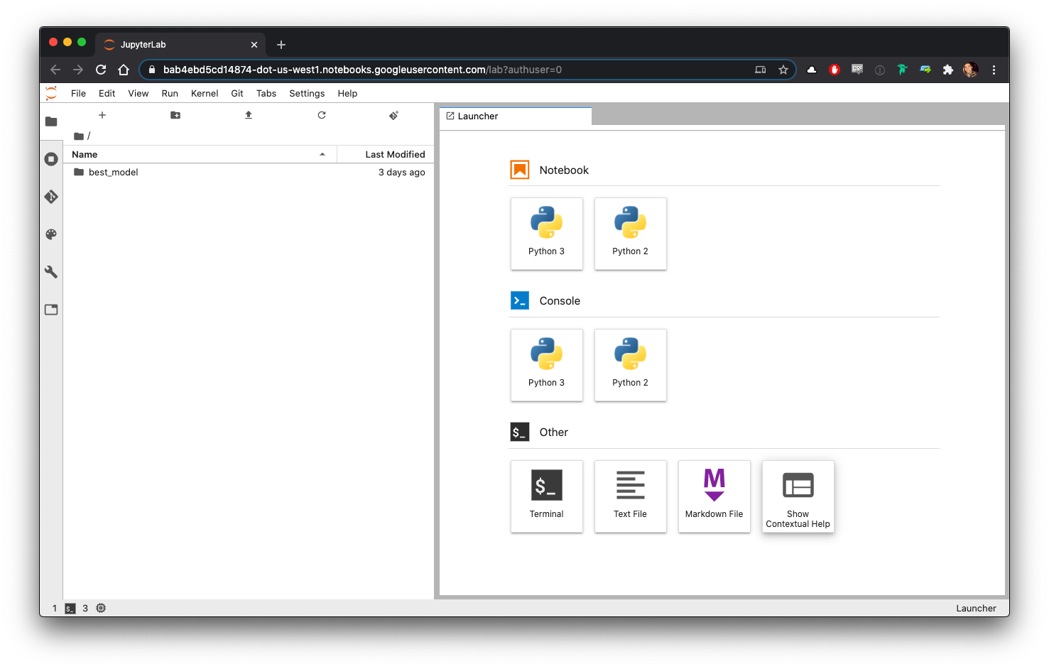
Within the saved model folder, there will be a saved_model.pb file, and folders for model assets and variables. The contents of these folders will change depending on the specifics of the changed model — however, we will be uploading this entire folder to CoS.

在保存的模型文件夹中，将有一个saved_model.pb文件以及用于模型资产和变量的文件夹。 这些文件夹的内容将根据更改模型的具体情况而有所不同-但是，我们会将整个文件夹上载到CoS。

The most convenient way to move the model folder is to use the Google Cloud Storage Python library.

移动模型文件夹最方便的方法是使用Google Cloud Storage Python库。

Before we begin, it’s worth noting that the storage library natively uploads one file at a time. Since the saved model consists of multiple files, in various folders, we will need to write a small function to recursively work through the folder and upload each file, maintaining the original file structure.

在开始之前，值得注意的是存储 库本机一次上载一个文件 。 由于保存的模型包含多个文件，因此位于不同的文件夹中，我们将需要编写一个小函数来递归遍历该文件夹并上载每个文件，并保持原始文件结构。

Using the code snippet below, write the function, and then upload the folder.

使用下面的代码片段，编写函数，然后上传文件夹。

from google.cloud import storage
import glob
import os


bucket_name = <<YOUR-BUCKET-NAME>>


def upload_folder(bucket_name, folder_path, destination_path):
    """
    Uploads an entire local folder to a Google Cloud Object Storage Bucket maintaining directly structure.
    """
    storage_client = storage.Client()
    bucket = storage_client.bucket(bucket_name)
    # Ensure that folder_path is a directory and not a file
    assert os.path.isdir(folder_path)
    
    for local_file in glob.glob(folder_path + '/**'):
        # Check if item in directory is a file, if it's not a file it is a folder and the upload_folder function is called recursively.
        if not os.path.isfile(local_file):
            upload_folder(bucket_name, local_file, destination_path+"/"+os.path.basename(local_file))
        else:
            # Create the remote path by joining the destination path and the base name of the local file
            remote_path = os.path.join(destination_path, local_file[1+len(folder_path):])
            blob = bucket.blob(remote_path)
            blob.upload_from_filename(local_file)


# Upload model to bucket
upload_folder(bucket_name, <<LOCAL_PATH>>, <<DESTINATION_PATH>>)
# Note - local path refers to the folder where the model was saved locally (e.g. model_keras/). Destination path refers
# to the folder where it should be uploaded to. You do not need to create a DESTINATION folder ahead of time. If you
# supply a path to a folder that doesn't exist - it will be created automatically.

You can verify that the upload has worked correctly by clicking into your storage bucket in the cloud console and looking for the uploaded folder.

您可以通过在云控制台中单击存储桶并查找上载的文件夹来验证上载是否正常工作。

Look in Storage > Browser to see all of your created buckets

在“存储”>“浏览器”中查看所有已创建的存储桶

After the model is successfully uploaded, we can move on to deployment.

成功上传模型后，我们可以继续进行部署。

创建一个新的模型和版本 (Create a New Model and Version)

Navigate to the AI Platform section in the Cloud Console and go to the Models page. Create a new model by clicking the New Model button at the top of the page.

导航到Cloud Console中的“ AI平台”部分，然后转到“模型”页面。 通过单击页面顶部的“新建模型”按钮来创建新模型。

You can always get the AI Platform and AI Platform Models screens using the hamburger menu at the top left of the screen.

您始终可以使用屏幕左上方的汉堡包菜单获取“ AI平台”和“ AI平台模型”屏幕。

An important point to understand: in the AI Platform, a Model holds many different Versions. The idea is that since model development and usage is iterative (e.g. retraining), it is expected that there will be many different versions of the same model and that we may want to keep and use older versions.

需要了解的重要一点：在AI平台中，模型包含许多不同的版本。 这个想法是，由于模型的开发和使用是迭代的(例如，重新训练)，因此可以预期，同一模型将有许多不同的版本，并且我们可能希望保留和使用较旧的版本。

The saved model file from the last tutorial will actually be a Version in the newly created model. This is why we did not have to specify the location of any of the files when it was created.

从上个教程保存的模型文件实际上是一个版本在新创建的模型。 这就是为什么我们在创建文件时不必指定任何文件的位置的原因。

After you’ve created the model, open the Model Details page from the Models page. Create a new version by clicking the New Version button at the top of the page.

创建模型后，从“模型”页面打开“模型详细信息”页面。 通过单击页面顶部的“新版本”按钮来创建新版本。

This tutorial involves a TensorFlow model, but it’s worth noting you can also deploy scikit-learn, XGBoost, and Custom Prediction Routines as well.

本教程涉及TensorFlow模型，但值得注意的是，您也可以部署scikit-learn，XGBoost和自定义预测例程。

Important Note: We suggest unticking the option to use a regional endpoint when creating your model for the purposes of this tutorial. If you do not, you will need to use whichever endpoint was selected during the creation process. Don’t worry — you can easily retrieve this later on!

重要说明：出于本教程的目的，建议不要在创建模型时取消使用区域端点的选项。 如果不这样做，则将需要使用在创建过程中选择的任何端点。 不用担心-您以后可以轻松检索到它！

Make sure to select the correct bucket from the list!

确保从列表中选择正确的存储桶！

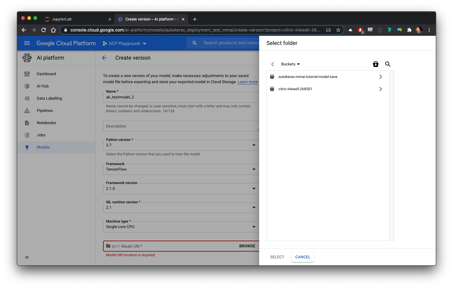
The location of the model files needs to be specified. If you don’t see your storage bucket in the folder browser, ensure that you have created the bucket in the same project as the AI Platform Model, and that you have selected the appropriate region for the bucket to be created in (i.e. the same region or multi-region space as your project and model).

需要指定模型文件的位置。 如果在文件夹浏览器中看不到存储桶，请确保已在与AI平台模型相同的项目中创建了存储桶，并确保选择了要在其中创建存储桶的适当区域(即，相同的区域)。区域或多区域空间作为您的项目和模型)。

Now that the model is deployed, we are ready to start making API requests to get predictions.

现在已经部署了模型，我们准备开始发出API请求以获取预测。

使用Postman和REST API进行预测 (Call for Predictions Using Postman and REST APIs)

For this tutorial, we will use Postman to make API requests. You can use whichever software you are most comfortable with to make the requests, including the Python Requests library.

在本教程中，我们将使用Postman发出API请求。 您可以使用最喜欢的软件来发出请求，包括Python Requests库。

Postman is a platform for API development and testing. It is simple to use, and widely used in industry. Download and install the version of Postman that is most appropriate for your system — they offer versions Windows, macOS and Linux.

Postman是用于API开发和测试的平台。 它使用简单，并在工业中广泛使用。 下载并安装最适合您的系统的Postman版本-他们提供Windows，macOS和Linux版本。

Now that you have Postman ready to go — let’s move back to the AI Platform Notebook and get a few pieces of information needed to make API calls.

既然您已经准备好邮递员了-让我们回到AI平台笔记本上，获取进行API调用所需的一些信息。

First, we will need to get an authentication key. To do so, run the following code in a Jupyter Notebook cell and copy the returned token string:

首先，我们将需要获取验证密钥。 为此，请在Jupyter Notebook单元中运行以下代码，然后复制返回的令牌字符串：

!gcloud auth application-default print-access-token

Note: this is not a very secure or persistent way of authenticating — it will time out after a few minutes. OAuth authentication is recommended for deployments that consume or return sensitive information, but are beyond the scope of this tutorial.

注意：这不是一种非常安全或持久的身份验证方法- 几分钟后会超时 。 对于使用或返回敏感信息的部署，建议使用OAuth身份验证，但不属于本教程的范围。

The main endpoint for API calls related to this model and project is:

与该模型和项目相关的API调用的主要端点是：

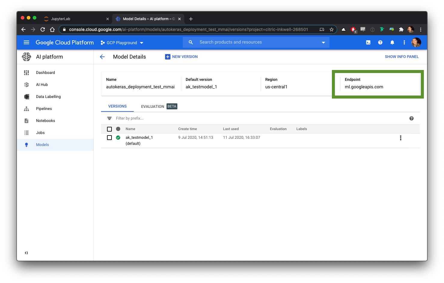
https://ml.googleapis.com

Reminder: If you used a regional endpoint when creating your model, you will need to replace the above URL with the endpoint found on your model’s details page.

提醒：如果在创建模型时使用了区域端点，则需要用模型详细信息页面上的端点替换上述URL。

Look in the green box for the model’s endpoint

在绿色框中查找模型的端点

We will specify the model, but not specify a version since we only have one. If you have multiple versions, it will pick the default version, or you can specify which version should be used in the inference.

我们将指定模型，但不指定版本，因为我们只有一个。 如果有多个版本，它将选择默认版本，或者您可以指定在推断中使用哪个版本。

We will be making online predictions. Online predictions are inferenced immediately and returned synchronously. There are also options to make batch predictions. However, this requires uploading the input data to CoS before calling for predictions. In this tutorial, we want to focus on sending input data as part of the predictions request. More information can be found in the Google documentation.

我们将进行在线预测。 在线预测将立即被推断并同步返回。 还有一些选项可以进行批量预测。 但是，这需要在调用预测之前将输入数据上载到CoS。 在本教程中，我们要集中精力发送输入数据作为预测请求的一部分。 可以在Google文档中找到更多信息。

We will be using the projects.predict method to call for predictions; this is worth a quick glance.

我们将使用projects.predict方法进行预测； 值得一看。

Open up Postman and start creating a new request.

打开Postman并开始创建一个新请求。

You can start a new request by clicking the orange “New” button at the top left, or in the grey-lighted box towards the centre of the screen

您可以通过点击左上角的橙色“新建”按钮，或在屏幕中央的灰色方框中启动新请求

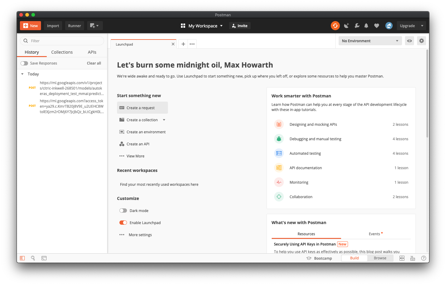
As seen in the Google documentation, this is a POST request. Change the request type from GET to POST.

如Google文档所示，这是一个POST请求。 将请求类型从GET更改为POST。

Use the dropdown in the green box to switch the request type from GET to POST

使用绿色框中的下拉列表将请求类型从GET切换为POST

The full URL of predict API is:

预测API的完整URL为：

https://ml.googleapis.com/v1/projects/your-project-id/models/your-model-name:predict

Where “your-project-id” and “your-model-name” are your project id and model name, respectively.

其中“您的项目ID”和“您的模型名称”分别是您的项目ID和模型名称。

Pro-Tip: To get your your project ID click on the name of the project at the top of the page. An overlay will appear containing a list of your projects by name and ID. You want the ID, not the name! See the green box in the image below.

专家提示：要获取您的项目ID，请点击页面顶部的项目名称。 将出现一个覆盖，其中包含按名称和ID列出的项目列表。 您想要的是ID， 而不是名称！ 请参见下图中的绿色框。

Pro-Tip: To get your model name you can navigate to the Models page in your AI Platform console.

专家提示：要获取模型名称，您可以导航到AI Platform控制台中的“模型”页面。

After replacing your information in the above URL (i.e. your-project-id and your-model-name) copy and paste it into the request URL box — see the green box in the image below.

在将您的信息替换为上述URL(即your-project-id和your-model-name )后，将其复制并粘贴到请求URL框中-请参见下图中的绿色框。

Next, we will need to add the token we generated a little earlier. In the “Params” tab, add a new parameter with key = access_token and value = the copied token — see the purple box in the image below.

接下来，我们需要添加之前生成的令牌。 在“参数”选项卡中，添加一个新参数，其键为= access_token ， 值=复制的令牌 —请参见下图的紫色框。

Copy the endpoint URL with your-project-id and your-model-name into the green box. Copy the access_token into the purple box.

将带有your-project-id和your-model-name的端点URL复制到绿色框中。 将access_token复制到紫色框中。

Finally, we need to prepare some data to test the API. We will use some of the same test data that was used during training.

最后，我们需要准备一些数据来测试API。 我们将使用与培训期间相同的测试数据。

An additional note on online predictions: the maximum size of the data payload is 1.5MB. For image classification, this may present an issue; however, there are several well-documented strategies to compress the image data more efficiently.

有关在线预测的其他说明： 数据有效负载的最大大小为1.5MB 。 对于图像分类，这可能会带来问题； 但是，有许多文献记载的策略可以更有效地压缩图像数据。

For example, in this tutorial, the saved model is expecting images to be input as Numpy arrays. However, we could modify this so that it accepts base64 encoded images (~60X smaller file sizes), or by sending a URL where the image is downloaded from prior to inferencing.

例如，在本教程中，保存的模型期望图像作为Numpy数组输入。 但是，我们可以对其进行修改，以使其接受base64编码的图像(小60倍左右的文件大小)，或者通过发送URL进行推断，从该URL下载图像。

An additional option is to upload the image file to CoS, and then call for batch predictions. This tutorial focuses on online predictions only, but it is not a significant leap to switch strategies.

另一个选择是将图像文件上传到CoS，然后调用批量预测 。 本教程仅关注在线预测 ，但切换策略并不是重大的飞跃。

As with most REST requests, our data payload will conform to a specific JSON format:

与大多数REST请求一样，我们的数据有效载荷将遵循特定的JSON格式：

{"instances" : [
     {"input_1" :  <<Image_Array>>}
  ]}

For more information on formatting various different types of data for the online prediction API, see the Google Cloud documentation.

有关格式化在线预测API的各种不同类型的数据的更多信息，请参阅Google Cloud文档 。

To generate a suitable payload, we can simply dump the image data into a JSON file with the specified format, and then copy/paste this image data into Postman.

为了生成合适的有效负载，我们可以简单地将图像数据转储为具有指定格式的JSON文件，然后将该图像数据复制/粘贴到Postman中。

Use the code snippet below in your AI Platform notebook to generate a appropriate data payload to be copied into Postman.

在AI Platform笔记本中使用下面的代码段生成适当的数据有效载荷，以将其复制到Postman中。

import json
import numpy as np
import tensorflow as tf
import tensorflow_datasets as tfds


def prepare_payload(image_array, outfile_path):
  json_data = {"instances": [{"input_1":image_array}]}
  with open(outfile_path, "w") as outfile: 
    json.dump(json_data, outfile)
    
# Note - we will be using the x_test and y_test arrays that were created earlier in the tutorial to train the model
prepare_payload(X_test[1].tolist(), "data_payload.txt")

You should now be able to open the file directly in JupyterLab and copy and paste it into Postman.

现在，您应该能够直接在JupyterLab中打开文件并将其复制并粘贴到Postman中。

You can select the whole data payload by clicking anywhere in the opened document and selecting all (⌘+A or Ctrl-A)

您可以通过单击打开的文档中的任意位置并选择全部(⌘+ A或Ctrl-A)来选择整个数据负载

In Postman, open up the Body tab, select the “raw” radio button, and specify the format of the payload as JSON.

在Postman中，打开“正文”选项卡，选择“原始”单选按钮，然后将有效负载的格式指定为JSON。

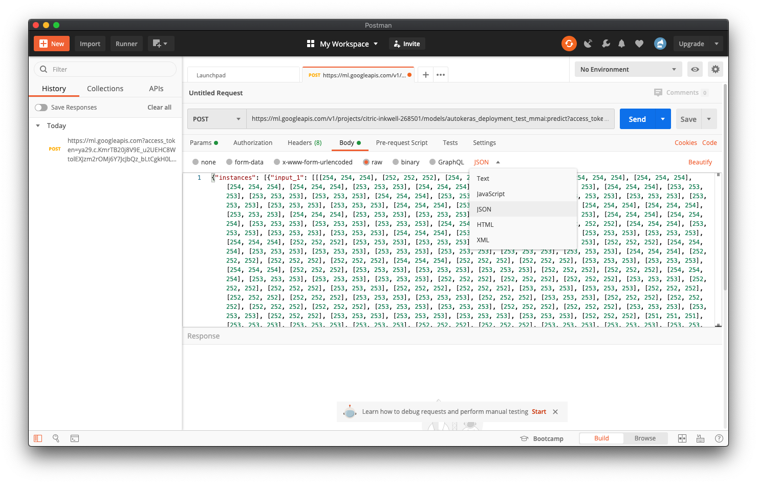
You can copy and paste the contents of the newly created JSON file directly into Postman, and click send.

您可以将新创建​​的JSON文件的内容直接复制并粘贴到Postman中，然后单击发送。

You should quickly get a response with a JSON object containing the results of the predictions.

您应该使用包含预测结果的JSON对象快速获得响应。

Note: A compute node must be spun up to handle your inference request. If you are testing during a busy time, or if it’s the first time calling for an inference in a while, it may take a bit of extra time to bring a node online.

注意：必须旋转计算节点才能处理您的推理请求。 如果在繁忙时间进行测试，或者这是一段时间以来第一次进行推理，则可能需要花费一些额外的时间才能使节点联机。

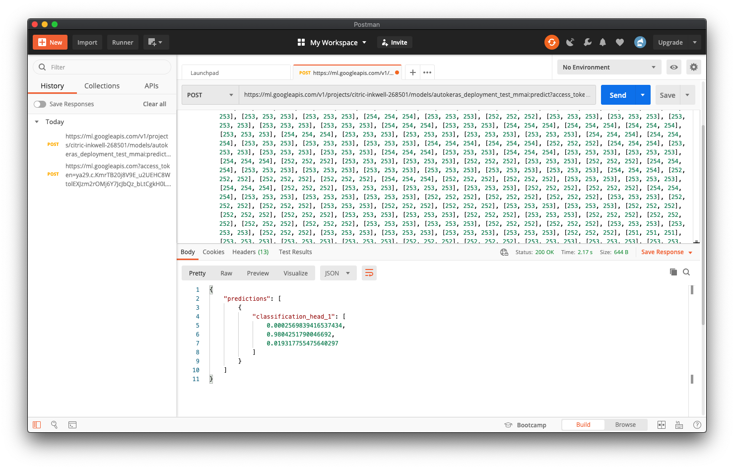
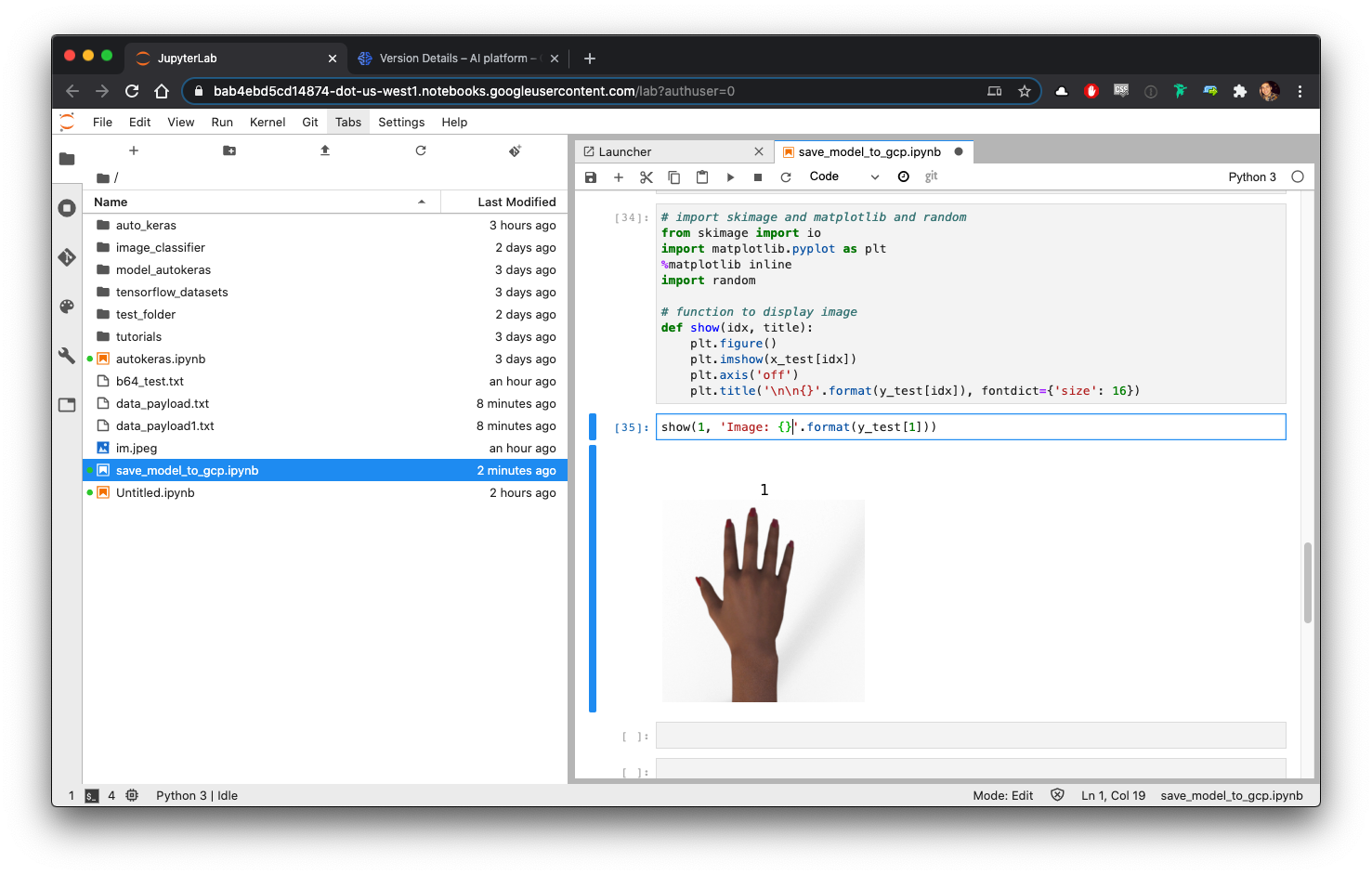
In this case, we can see that the model has predicted this to be a “Paper” move. Let’s take a quick look at the image and it’s label to see if this was correct!

在这种情况下，我们可以看到模型已预测这是“纸”动作。 让我们快速浏览一下图片和标签，看看这是否正确！

from skimage import io
import matplotlib.pyplot as plt
%matplotlib inline


# function to display image
# note that this function is hard coded to refer to the test images and labels - please modify accordingly. 
def show(idx, title):
    plt.figure()
    plt.imshow(X_test[idx])
    plt.axis('off')
    plt.title('\n\n{}'.format(y_test[idx]), fontdict={'size': 16})
    
show(1, 'Image: {}'.format(y_test[1]))

Looking at the results, we can see that the predictions were correct!

查看结果，我们可以看到预测是正确的！

A vast range of functionality is available through the REST APIs, including creating and training new model versions, which allows for generous model management capabilities from a variety of different devices in many different operating scenarios.

REST API提供了广泛的功能，包括创建和训练新的模型版本，从而允许在许多不同的操作场景中使用来自各种不同设备的大量模型管理功能。

专家提示：将GPU连接到笔记本 (Pro-Tip: Attaching GPUs to your Notebook)

To allocate GPU resources, you need first to have a GPU quota that is not zero! You can request an increase in GPU quota by navigating to IAM & Admin > Quotas. Search for GPUs (all regions) in the Filter table region.

要分配GPU资源，首先需要拥有不为零的GPU配额！ 您可以通过导航到IAM＆Admin> Quotas来请求增加GPU 配额 。 在“ 过滤器”表区域中搜索GPU(所有区域) 。

This screenshot shows my GPUs (all regions) quote as 1 for the project.

此屏幕快照显示了我的GPU(所有区域)在项目中的报价为1。

Select the GPUs (all regions) quota and click Edit Quotas.

选择GPU(所有区域)配额，然后点击编辑配额 。

Note — If you cannot select the quota, and you have a “Upgrade Account” banner at the top of the window, you will need to upgrade and then refresh the page before you can select the quota to edit.

注 —如果无法选择配额，并且窗口顶部显示“ Upgrade Account”(升级帐户)标语，则需要先升级然后刷新页面，然后才能选择要编辑的配额。

Follow the steps to fill in the request form to increase your quota. It can take anywhere from a few hours to a few days for a quota to be approved. We suggest only requesting an increase of 1 GPU.

请按照以下步骤填写申请表，以增加配额。 批准配额可能需要几个小时到几天的时间。 我们建议仅请求增加1个GPU。

With your AI Notebooks VM stopped, you can now attach a GPU resource to the VM by selecting it in the dropdown.

在AI Notebooks VM停止的情况下，现在可以通过在下拉列表中选择GPU资源来将GPU资源附加到VM。

Attaching a GPU resource to a shutdown AI Notebooks VM.

将GPU资源附加到已关闭的AI Notebooks VM。

You will now need to install the appropriate NVIDIA driver to run talk to the GPU. Run the steps on this page in a terminal (launched from JupyterLab) for the best results. Another convenient way to do it is just to create a new VM and check the Install NVIDIA GPU driver automatically for me box.

现在，您需要安装适当的NVIDIA驱动程序以与GPU进行对话。 在终端(从JupyterLab启动)中运行此页面上的步骤以获得最佳结果。 另一种方便的方法是创建一个新的VM，然后选中“ 自动为我安装NVIDIA GPU”框。

Finally, we will also have to do a pip uninstall for tensorflow and replace it with tensorflow-gpu.

最后，我们还必须对tensorflow进行pip卸载并将其替换为tensorflow-gpu。

pip uninstall tensorflow
pip install tensorflow-gpu

结论 (Conclusion)

Neural Architecture Search (NAS) methods are set to become a necessary part of Deep Learning initiatives quickly. They provide a significant advantage over traditional grid search or, more likely, trial and error based architecture optimization.

神经体系结构搜索(NAS)方法将很快成为深度学习计划的必要组成部分。 与传统的网格搜索或更可能是基于试验和错误的体系结构优化相比，它们具有明显的优势。

Although tools like AutoML are now widely available, their cost makes implementing prohibitive for many use cases.

尽管诸如AutoML之类的工具现在已广泛使用，但其成本使得实现许多用例望而却步。

In this tutorial, we’ve shown how you can use freely available NAS packages like Auto-Keras on the Google Cloud AI Platform to build a custom CNN architecture that is optimized for a specific dataset and use case. You also now know how to take that model, and deploy it to a production-ready environment, and call for predictions on image data using REST APIs.

在本教程中，我们展示了如何在Google Cloud AI平台上使用免费的NAS程序包(例如Auto-Keras)来构建针对特定数据集和用例进行优化的自定义CNN架构。 您现在还知道如何采用该模型，并将其部署到可用于生产的环境中，并使用REST API要求对图像数据进行预测。

This tutorial was written and developed by Team Watts, part of the Queen’s University MMAI program at Smith in Toronto, Ontario.

本教程由 Team Watts 编写和开发，该 团队 是位于 安大略省多伦多市Smith 的 女王大学MMAI计划的 一部分 。

翻译自: https://medium.com/team-watts/automl-diy-edition-60449b24f7

automl