


目录:(Table of Contents:)
1.简介(1. Introduction)
Neural machine translation (NMT) is an approach to machine translation that uses an artificial neural network to predict the likelihood of a sequence of words, typically modeling entire sentences in a single integrated model.
神经机器翻译(NMT)是一种机器翻译方法,它使用人工神经网络来预测单词序列的可能性,通常在单个集成模型中对整个句子进行建模。
It was one of the hardest problems for computers to translate from one language to another with a simple rule-based system because they were not able to capture the nuances involved in the process. Then shortly we were using statistical models but after the entry of deep learning the field is collectively called Neural Machine Translation and now it has achieved State-Of-The-Art results.
使用基于规则的简单系统将计算机从一种语言转换为另一种语言是最困难的问题之一,因为它们无法捕获过程中涉及的细微差别。 然后不久我们就使用了统计模型,但是在深度学习开始后,该领域统称为神经机器翻译,现在它已经取得了最新的成果。
I want this post to be beginner-friendly, so a specific kind of architecture (Seq2Seq) showed a good sign of success, is what we are going to implement here.
我希望这篇文章对初学者友好,因此我们将在此处实现的一种特定体系结构(Seq2Seq)显示出成功的好兆头。
So the Sequence to Sequence (seq2seq) model in this post uses an encoder-decoder architecture, which uses a type of RNN called LSTM (Long Short Term Memory), where the encoder neural network encodes the input language sequence into a single vector, also called as a Context Vector.
因此,本文中的序列到序列(seq2seq)模型使用了编码器-解码器体系结构,该体系结构使用一种称为LSTM(长短期记忆)的RNN,其中编码器神经网络将输入语言序列编码为单个矢量,称为上下文向量。
This Context Vector is said to contain the abstract representation of the input language sequence.
据说此文本向量包含输入语言序列的抽象表示。
This vector is then passed into the decoder neural network, which is used to output the corresponding output language translation sentence, one word at a time.
然后将此向量传递到解码器神经网络,该网络用于输出对应的输出语言翻译语句,一次输出一个单词。
Here I am doing a German to English neural machine translation. But the same concept can be extended to other problems such as Named Entity Recognition (NER), Text Summarization, even other language models, etc.
在这里,我正在做德语到英语的神经机器翻译。 但是相同的概念可以扩展到其他问题,例如命名实体识别(NER),文本摘要,甚至其他语言模型等。
2.数据准备和预处理 (2. Data Preparation and Pre-processing)
For getting the data in the best way we want, I am using SpaCy (Vocabulary Building), TorchText (text Pre-processing) libraries, and multi30k dataset which contains the translation sequences for English, German and French languages
为了以我们想要的最佳方式获取数据,我正在使用SpaCy(词汇构建),TorchText(文本预处理)库和multi30k数据集,其中包含英语,德语和法语的翻译序列
Torch text is a powerful library for making the text data ready for a variety of NLP tasks. It has all the tools to perform preprocessing on the textual data.
火炬文本是一个强大的库,用于使文本数据为各种NLP任务做好准备。 它具有用于对文本数据执行预处理的所有工具。
Let’s see some of the processes it can do,
让我们看看它可以做的一些过程,
1. Train/ Valid/ Test Split: partition your data into a specified train/ valid/ test set.
1.训练/有效/测试拆分:将数据划分为指定的训练/有效/测试集。
2. File Loading: load the text corpus of various formats (.txt,.json,.csv).
2.文件加载:加载各种格式(.txt,.json,.csv)的文本语料库。
3. Tokenization: breaking sentences into a list of words.
3.标记化:将句子分成单词列表。
4. Vocab: Generate a list of vocabulary from the text corpus.
4.翻译:由该文本语料库词汇的列表。
5. Words to Integer Mapper: Map words into integer numbers for the entire corpus and vice versa.
5.单词到整数映射器:将单词映射为整个语料库的整数,反之亦然。
6. Word Vector: Convert a word from a higher dimension to a lower dimension (Word Embedding).
6.单词向量:将单词从较高维度转换为较低维度(词嵌入)。
7. Batching: Generate batches of the sample.
7.批处理:生成一批样品。
So once we get to understand what can be done in torch text, let’s talk about how it can be implemented in the torch text module. Here we are going to make use of 3 classes under torch text.
因此,一旦我们了解了在割炬文本中可以执行的操作,就让我们讨论如何在割炬文本模块中实现它。 在这里,我们将在火炬文本下使用3个类。
1. Fields :
1.栏位:
- This is a class under the torch text, where we specify how the preprocessing should be done on our data corpus. 这是手电筒文本下的一类,我们在其中指定如何对数据集进行预处理。
2. TabularDataset :
2. TabularDataset :
- Using this class, we can actually define the Dataset of columns stored in CSV, TSV, or JSON format and also map them into integers. 使用此类,我们可以实际定义以CSV,TSV或JSON格式存储的列的数据集,并将它们映射为整数。
3. BucketIterator :
3. BucketIterator :
- Using this class, we can perform padding our data for approximation and make batches with our data for model training. 使用此类,我们可以对数据进行填充以进行近似,并使用我们的数据进行批处理以进行模型训练。
Here our source language (SRC — Input) is German and the target language (TRG — Output) is English. We also add 2 extra tokens “start of sequence” <sos> and “end of sequence” <EOS> for effective model training.
在这里,我们的源语言(SRC-输入)是德语,目标语言(TRG-输出)是英语。 我们还添加了两个额外的令牌“序列开始” <sos>和“序列结束” <EOS>,以进行有效的模型训练。
After setting the language pre-processing criteria, the next step is to create batches of training, testing, and validation data using iterators.
设置语言预处理标准后,下一步是使用迭代器创建一批培训,测试和验证数据。
Creating batches is an exhaustive process, luckily we can make use of TorchText’s iterator library.
创建批处理是一个详尽的过程,幸运的是,我们可以使用TorchText的迭代器库。
Here we are using BucketIterator for effective padding of source and target sentences. We can access the source (german) batch of data using the .src attribute and it's corresponding (English) batch of data using the .trg attribute. Also, we can see the data before tokenizing it.
在这里,我们使用BucketIterator来有效填充源句子和目标句子。 我们可以使用.src属性访问源(德语)数据批次,而使用.trg属性访问相应的(英语)数据批次。 此外,我们可以在标记数据之前查看数据。
I just experimented with a batch size of 32 and a sample batch is shown below. The sentences are tokenized into a list of words and indexed according to the vocabulary. The “pad” token gets an index of 1.
我刚刚试验了32个批次,下面显示了一个示例批次。 句子被标记为单词列表,并根据词汇索引。 “填充”令牌的索引为1。
Each column corresponds to a sentence, indexed into numbers and we have 32 such sentences in a single target batch and the number of rows corresponds to the maximum length of that sentence. Short sentences are padded with 1's to compensate for the length.
每列对应一个句子,索引成数字,我们在一个目标批次中有32个这样的句子,行数对应于该句子的最大长度。 短句用1填充以补偿长度。
The table below (Idx.csv) contains the numerical indices of the batch, which is later fed into the word embedding and converted into dense representation for Seq2Seq processing.
下表(Idx.csv)包含该批次的数字索引,该索引随后被馈送到单词嵌入中,并转换为用于Seq2Seq处理的密集表示形式。
The table below (Words.csv) contains the corresponding words mapped with the numerical indices of the batch.
下表(Words.csv)包含与批次的数字索引对应的对应单词。
3.长期短期记忆(LSTM)(3. Long Short Term Memory (LSTM))
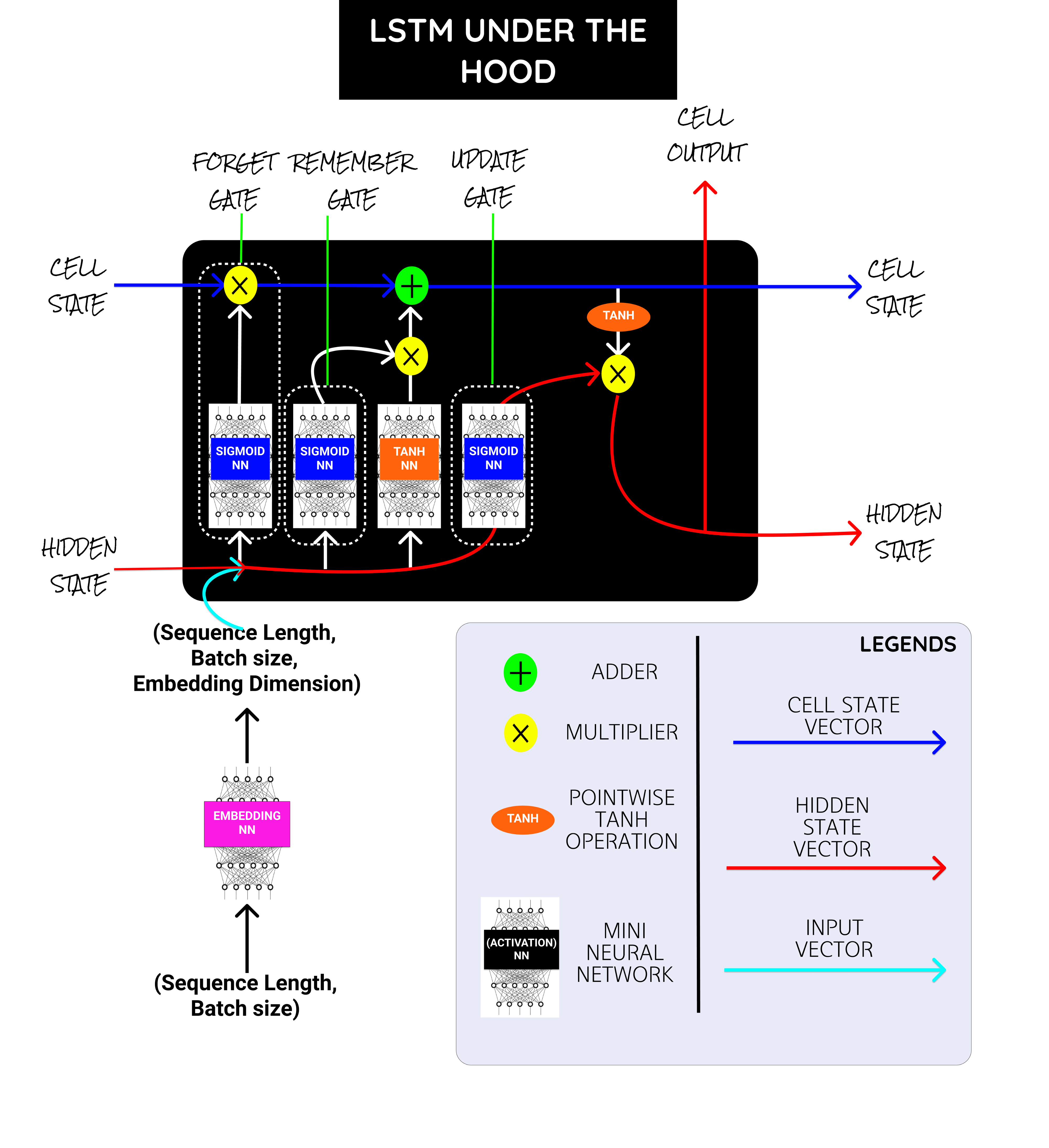
The above picture shows the units present under a single LSTM Cell. I will add some references to learn more about LSTM in the last and why it works well for long sequences.
上图显示了单个LSTM单元下的单位。 我将添加一些参考资料,以在最后了解更多有关LSTM的知识,以及为什么它对长序列有效。
But to simply put, Vanilla RNN, Gated Recurrent Unit (GRU) is not able to capture the long term dependencies due to its nature of design and suffers heavily by the Vanishing Gradient problem, which makes the rate of change in weights and bias values negligible, resulting in poor generalization.
但是简单地说,由于其设计的性质,Vanilla RNN门控循环单元(GRU)无法捕获长期依赖关系,并且遭受Vanishing Gradient问题的严重困扰,这使得权重和偏差值的变化率可忽略不计,导致泛化不佳。
Inside the LSTM cell, we have a bunch of mini neural networks with sigmoid and TanH activations at the final layer and few vector adder, Concat, multiplications operations.
在LSTM单元内部,我们有一堆微型神经网络,它们的最后一层具有S型和TanH激活,并且很少进行矢量加法器,Concat和乘法运算。
Sigmoid NN → Squishes the values between 0 and 1. Say a value closer to 0 means to forget and a value closer to 1 means to remember.
乙状结肠 →压缩介于0和1之间的值。说接近0的值表示忘记,而接近1的值表示记住。
Embedding NN → Converts the input word indices into word embedding.
嵌入NN →将输入的单词索引转换为单词嵌入。
TanH NN → Squishes the values between -1 and 1. Helps to regulate the vector values from either getting exploded to the maximum or shrank to the minimum.
TanH NN →压缩-1和1之间的值。有助于调节矢量值,使其免于爆炸至最大值或缩小至最小值。
盖茨: (Gates:)
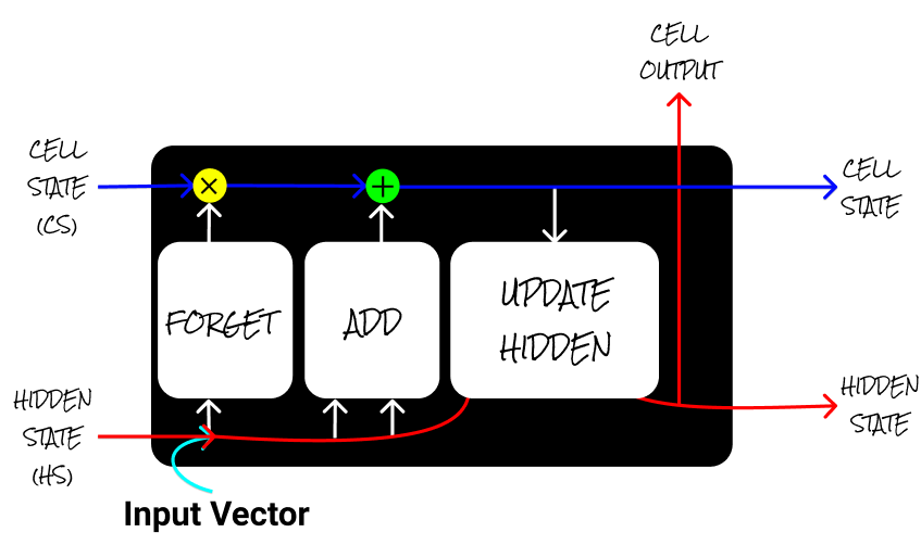
But LSTM has some special units called gates (Remember (Add) gate, Forget gate, Update gate), which helps to overcome the problems stated before.
但是LSTM有一些称为门的特殊单元(记住(添加)门,忘记门,更新门),这有助于克服前面提到的问题。
Forget Gate → Has sigmoid activation in it and range of values between (0–1) and it is multiplied over the cell state to forget some elements. (“Vector” * 0 = 0)
忘记门→具有S型激活,其值范围介于(0–1)之间,并与单元状态相乘以忘记某些元素。 (“向量” * 0 = 0)
Add Gate → Has TanH activation in it and range of values between
添加门→激活了TanH,其值范围介于
(-1 to +1) and it is
(-1至+1),它是
added over the cell state to remember some elements. (“Vector” * 1= “Vector”)
添加到单元格状态以记住一些元素。 (“向量” * 1 =“向量”)
Update Hidden → Updates the Hidden State based on the Cell State.
更新隐藏→根据单元状态更新隐藏状态。
The hidden state and the cell state are referred to here as the context vector, which are the outputs from the LSTM cell. The input is the sentence’s numerical indexes fed into the embedding NN.
隐藏状态和单元状态在这里称为上下文向量,它们是LSTM单元的输出。 输入是输入到嵌入NN中的句子的数字索引。
4.编码器模型架构(Seq2Seq) (4. Encoder Model Architecture (Seq2Seq))
Before moving to build the seq2seq model, we need to create an Encoder, Decoder, and create an interface between them in the seq2seq model.
在开始构建seq2seq模型之前,我们需要创建一个Encoder,Decoder,并在seq2seq模型中创建它们之间的接口。
Let’s pass the german input sequence “Ich Liebe Tief Lernen” which translates to “I love deep learning” in English.
让我们通过德语输入序列“ Ich Liebe Tief Lernen ”,该序列翻译成英语的“我爱深度学习”。
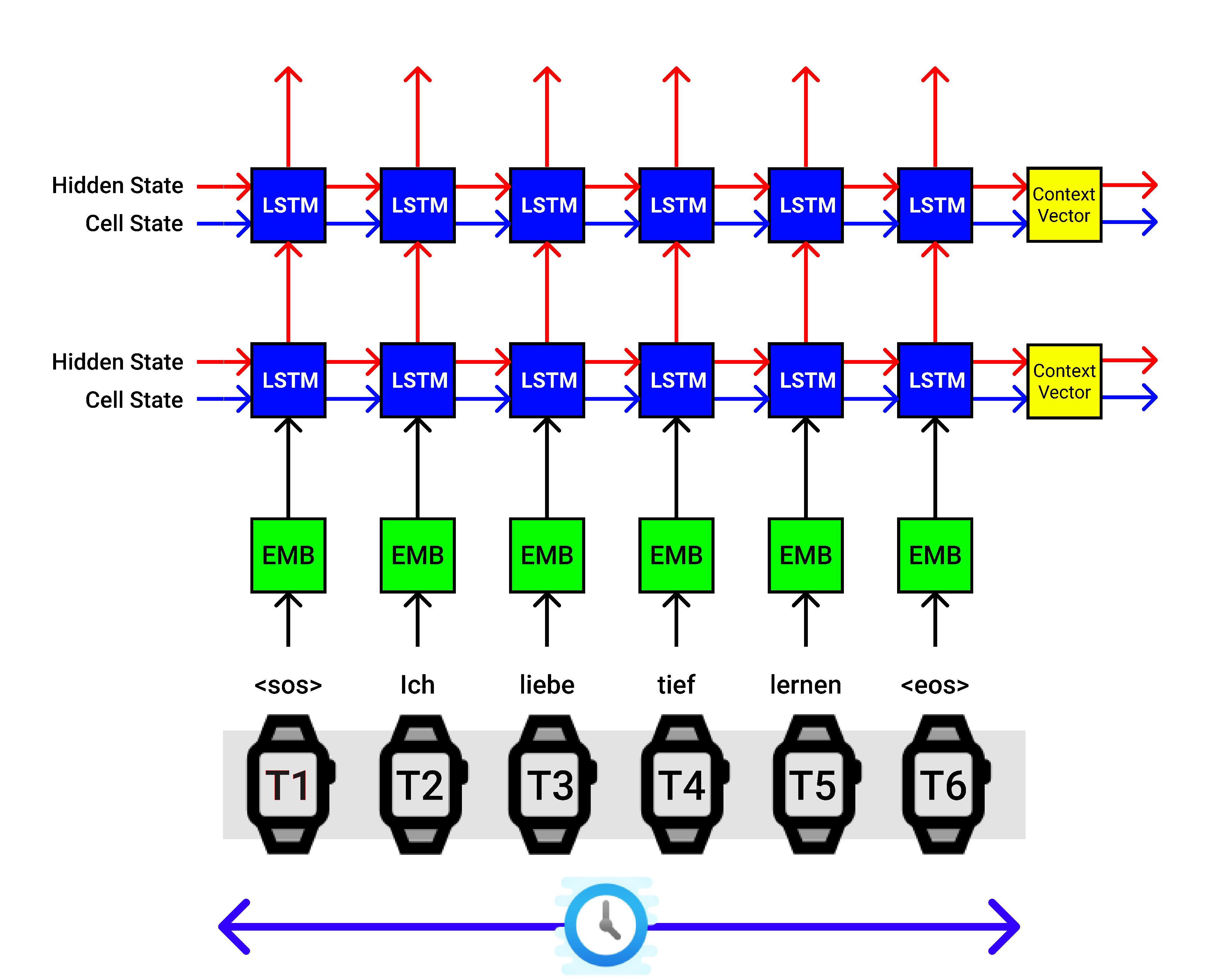
For a lighter note, let’s explain the process happening in the above image. The Encoder of the Seq2Seq model takes one input at a time. Our input German word sequence is “ich Liebe Tief Lernen”.
为了便于说明,让我们解释上图中发生的过程。 Seq2Seq模型的编码器一次只接受一个输入。 我们输入的德语单词序列为“ ich Liebe Tief Lernen”。
Also, we append the start of sequence “SOS” and the end of sentence “EOS” tokens in the starting and in the ending of the input sentence.
另外,我们在输入句子的开头和结尾处附加序列“ SOS”的开头和句子“ EOS”标记的结尾。
Therefore at
因此在
- At time step-0, the ”SOS” token is sent,在时间步0,发送“ SOS”令牌,
- At time step-1 the token “ich” is sent, 在步骤1,令牌“ ich”被发送,
- At time step-2 the token “Liebe” is sent, 在时间步骤2,令牌“ Liebe”被发送,
- At time step-3 the token “Tief” is sent, 在步骤3中,发送了令牌“ Tief”,
- At time step-4 the token “Lernen” is sent, 在第4步,令牌“ Lernen”被发送,
- At time step-4 the token “EOS” is sent. 在时间步骤4,发送令牌“ EOS”。
And the first block in the Encoder architecture is the word embedding layer [shown in green block], which converts the input indexed word into a dense vector representation called word embedding (sizes — 100/200/300).
编码器体系结构中的第一个块是单词嵌入层(以绿色块显示),该层将输入的索引词转换为称为词嵌入的密集向量表示(大小为100/200/300)。
Then our word embedding vector is sent to the LSTM cell, where it is combined with the hidden state (hs), and the cell state (cs) of the previous time step and the encoder block outputs a new hs and a cs which is passed to the next LSTM cell. It is understood that the hs and cs captured some vector representation of the sentence so far.
然后我们的词嵌入向量被发送到LSTM单元,在这里它与隐藏状态(hs)组合,并且前一个时间步的单元状态(cs)组合,编码器块输出新的hs和cs到下一个LSTM单元。 可以理解,到目前为止,hs和cs捕获了该句子的某些矢量表示。
At time step-0, the hidden state and cell state are either initialized fully of zeros or random numbers.
在时间步-0,隐藏状态和单元状态被完全初始化为零或随机数。
Then after we sent pass all our input German word sequence, a context vector [shown in yellow block] (hs, cs) is finally obtained, which is a dense representation of the word sequence and can be sent to the decoder’s first LSTM (hs, cs) for corresponding English translation.
然后,在我们发送完所有输入的德语单词序列之后,最终获得上下文向量[以黄色块显示](hs,cs),该上下文向量是单词序列的密集表示形式,可以发送到解码器的第一个LSTM(hs ,cs)进行相应的英语翻译。
In the above figure, we use 2 layer LSTM architecture, where we connect the first LSTM to the second LSTM and we then we obtain 2 context vectors stacked on top as the final output. This is purely experimental, you can manipulate it.
在上图中,我们使用2层LSTM体系结构,其中将第一个LSTM连接到第二个LSTM,然后获得2个上下文向量,这些向量堆叠在顶部作为最终输出。 这纯粹是实验性的,您可以对其进行操作。
It is a must that we design identical encoder and decoder blocks in the seq2seq model.
我们必须在seq2seq模型中设计相同的编码器和解码器模块。
The above visualization is applicable for a single sentence from a batch.
以上可视化适用于批处理中的单个句子。
Say we have a batch size of 5 (Experimental), then we pass 5 sentences with one word at a time to the Encoder, which looks like the below figure.
假设我们的批处理大小为5(实验性),然后一次将5个句子(每个单词带有一个单词)传递给编码器,如下图所示。

5.编码器代码实现(Seq2Seq)(5. Encoder Code Implementation (Seq2Seq))
6.解码器模型架构(Seq2Seq) (6. Decoder Model Architecture (Seq2Seq))

The decoder also does a single step at a time.
解码器一次也执行单个步骤。
The Context Vector from the Encoder block is provided as the hidden state (hs) and cell state (cs) for the decoder’s first LSTM block.
提供来自编码器块的上下文向量,作为解码器的第一个LSTM块的隐藏状态(hs)和单元状态(cs)。
The start of sentence “SOS” token is passed to the embedding NN, then passed to the first LSTM cell of the decoder, and finally, it is passed through a linear layer [Shown in Pink color], which provides an output English token prediction probabilities (4556 Probabilities) [4556 — as in the total vocabulary size of English language], hidden state (hs), Cell State (cs).
句子“ SOS”令牌的开头被传递到嵌入的NN,然后传递到解码器的第一个LSTM单元,最后,它经过一个线性层[以粉红色显示],该层提供输出的英语令牌预测概率( 4556概率)[4556 —如英语的总词汇量一样],隐藏状态(hs),单元状态(cs)。
The output word with the highest probability out of 4556 values is chosen, hidden state (hs), and Cell State (cs) is passed as the inputs to the next LSTM cell and this process is executed until it reaches the end of sentences “EOS”.
选择4556个值中概率最高的输出单词,将隐藏状态(hs)和单元状态(cs)作为输入传递到下一个LSTM单元,并执行此过程,直到到达句子“ EOS”的结尾” 。
The subsequent layers will use the hidden and cell state from the previous time steps.
后续层将使用先前时间步骤中的隐藏状态和单元状态。
示教力比: (Teach Force Ratio:)
In addition to other blocks, you will also see the block shown below in the Decoder of the Seq2Seq architecture.
除其他块外,您还将在Seq2Seq架构的解码器中看到以下所示的块。
While model training, we send the inputs (German Sequence) and targets (English Sequence). After the context vector is obtained from the Encoder, we send them Vector and the target to the Decoder for translation.
在进行模型训练时,我们发送输入(德语序列)和目标(英语序列)。 从编码器获得上下文向量后,我们将它们和目标发送给解码器进行翻译。
But during model Inference, the target is generated from the decoder based on the generalization of the training data. So the output predicted words are sent as the next input word to the decoder until a <EOS> token is obtained.
但是在模型推断期间,目标是根据训练数据的一般性从解码器生成的。 因此,将输出的预测单词作为下一个输入单词发送到解码器,直到获得<EOS>令牌。
So in model training itself, we can use the teach force ratio (tfr), where we can actually control the flow of input words to the decoder.
因此,在模型训练本身中,我们可以使用示教力比(tfr) ,在这里我们可以实际控制输入字到解码器的流向。
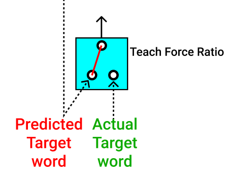
We can send the actual target words to the decoder part while training (Shown in Green Color).
我们可以在训练时将实际的目标词发送到解码器部分(以绿色显示)。
We can also send the predicted target word, as the input to the decoder (Shown in Red Color).
我们还可以发送预测的目标词,作为解码器的输入(以红色显示)。
Sending either of the word (actual target word or predicted target word) can be regulated with a probability of 50%, so at any time step, one of them is passed during the training.
发送单词(实际目标单词或预测目标单词)的可能性可以控制为50%,因此在任何时间步长,在训练过程中都会通过其中一个。
This method acts like a Regularization. So that the model trains efficiently and fastly during the process.
此方法的作用类似于正则化。 因此,在此过程中,模型可以快速有效地进行训练。
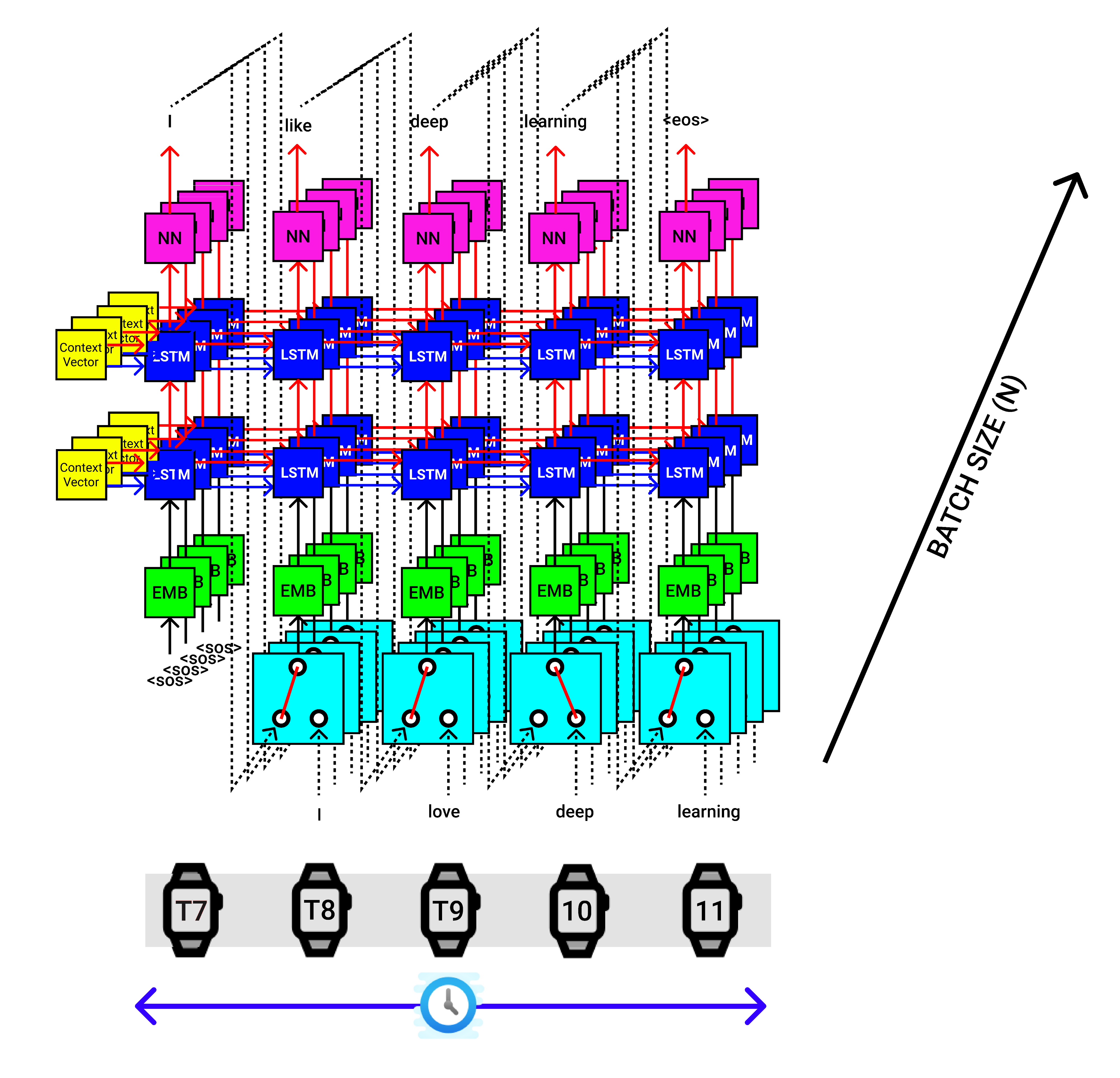
The above visualization is applicable for a single sentence from a batch. Say we have a batch size of 4(Experimental), then we pass 4sentences at a time to the Encoder, which provides 4 sets of Context Vectors, and they all are passed into the Decoder, which looks like the below figure.
以上可视化适用于批处理中的单个句子。 假设我们的批处理大小为4(实验性),然后一次将4个句子传递给编码器,该编码器提供4组上下文向量,它们都被传递到解码器中,如下图所示。
7.解码器代码实现(Seq2Seq)(7. Decoder Code Implementation (Seq2Seq))
8. Seq2Seq(编码器+解码器)接口 (8. Seq2Seq (Encoder + Decoder) Interface)
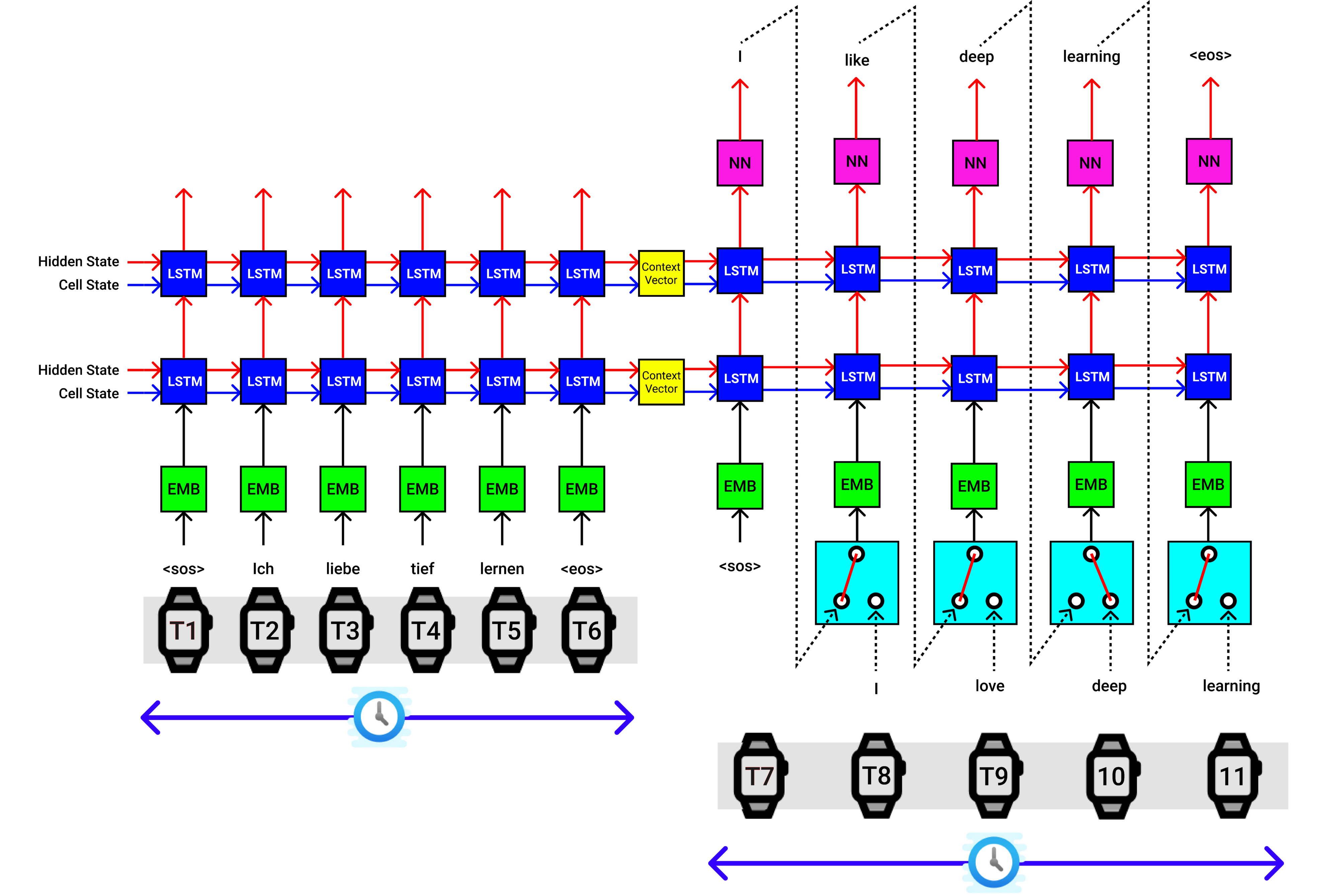
The final seq2seq implementation for a single input sentence looks like the figure below.
单个输入语句的最终seq2seq实现如下图所示。
- Provide both input (German) and output (English) sentences. 提供输入(德语)和输出(英语)句子。
Pass the input sequence to the encoder and extract context vectors.
将输入序列传递给编码器并提取上下文向量。
Pass the output sequence to the Decoder, context vectors from the Encoder to produce the predicted output sequence.
将输出序列传递给解码器,以及来自编码器的上下文向量,以生成预测的输出序列。
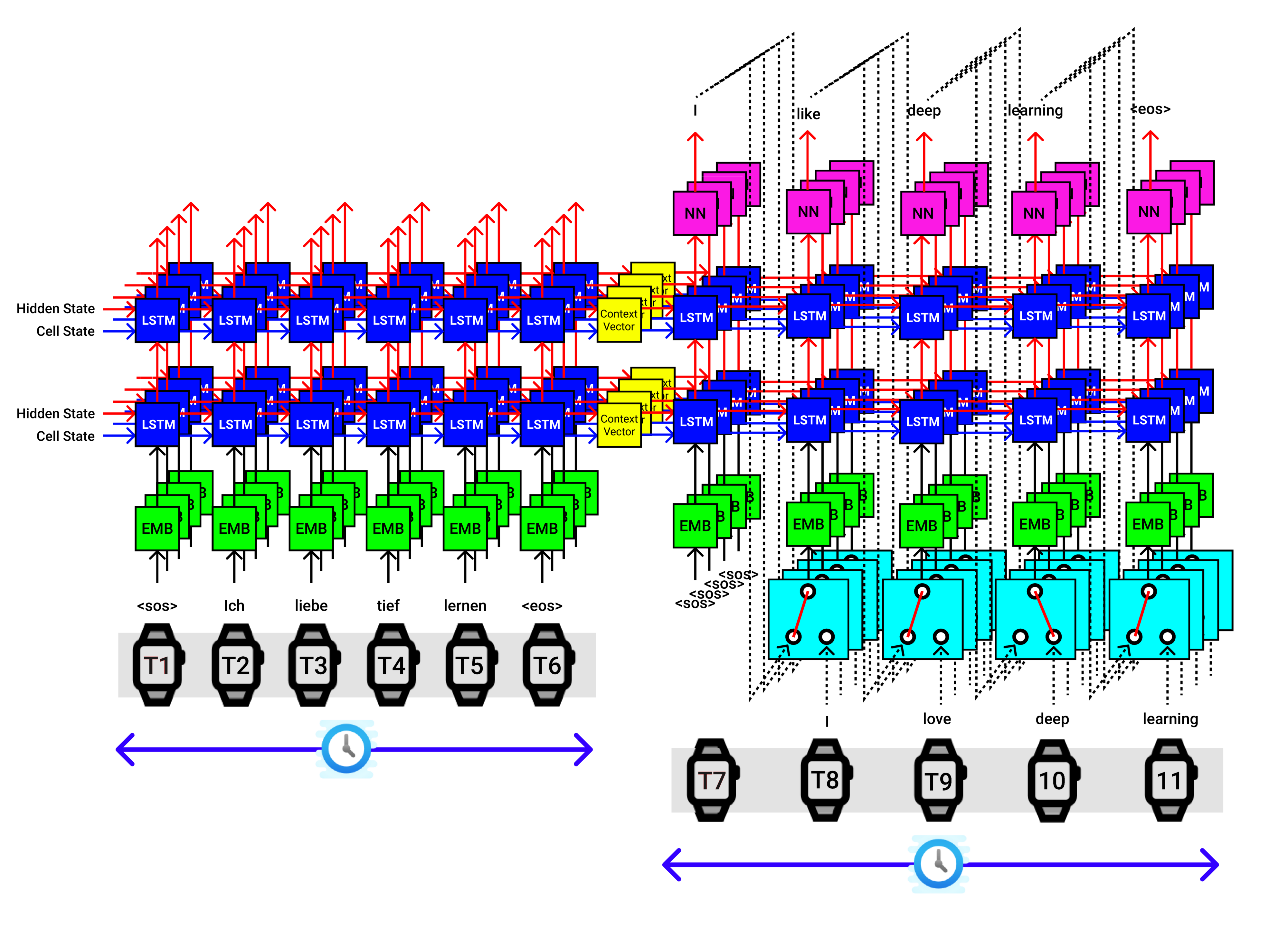
The above visualization is applicable for a single sentence from a batch. Say we have a batch size of 4 (Experimental), then we pass 4 sentences at a time to the Encoder, which provide 4 sets of Context Vectors, and they all are passed into the Decoder, which looks like the below figure.
以上可视化适用于批处理中的单个句子。 假设我们的批处理大小为4(实验性),然后一次将4个句子传递给编码器,该编码器提供4组上下文向量,它们都被传递到解码器中,如下图所示。
9. Seq2Seq(编码器+解码器)代码实现(9. Seq2Seq (Encoder + Decoder) Code Implementation)
10. Seq2Seq模型训练(10. Seq2Seq Model Training)
例句训练进度:(Training Progress for a sample sentence:)
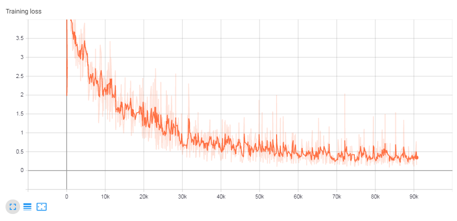
训练损失: (Training loss:)
11. Seq2Seq模型推论 (11. Seq2Seq Model Inference)
Now let us compare our trained model with that of SOTA Google Translate.
现在,让我们将我们训练有素的模型与SOTA Google Translate的模型进行比较。

Not bad, but clearly the model is not able to comprehend complex sentences. So in the upcoming series of posts, I will be enhancing the above model’s performance by altering the model’s architecture, like using Bi-directional LSTM, adding attention mechanism, or replacing LSTM with the Transformers model to overcome these apparent shortcomings.
不错,但是很明显,该模型不能理解复杂的句子。 因此,在接下来的系列文章中,我将通过更改模型的体系结构来提高上述模型的性能,例如使用双向LSTM,添加注意机制或用Transformers模型替换LSTM来克服这些明显的缺点。
12.资源和参考 (12. Resources & References)
I hope I was able to provide some visual understanding of how the Seq2Seq model processes the data, let me know your thoughts in the comment section.
希望我能够对Seq2Seq模型如何处理数据有一些直观的了解,在评论部分告诉我您的想法。
Check out the Notebooks that contains the entire code implementation and feel free to break it.
签出包含整个代码实现的笔记本,可以随意破坏它。
Complete Code Implementation is available at,
完整的代码实施可在以下网址获得:
@ GitHub
@ GitHub
@ Colab
@ Colab
@ Kaggle
@ Kaggle
For those who are curious, visualizations in this article were made possible by Figma & Google Drawing.
对于那些好奇的人, Figma和Google Drawing使本文中的可视化成为可能。
Complete Visualization files created on Figma (.fig) [LSTM, ENCODER+DECODER, SEQ2SEQ] is available @ Github.
在Github上可获得在Figma(.fig) [LSTM,ENCODER + DECODER,SEQ2SEQ]上创建的完整可视化文件。
References : LSTM, WORD_EMBEDDING, DEEP_LEARNING_MODEL_DEPLOYMENT_ON_AWS
参考文献: LSTM , WORD_EMBEDDING , DEEP_LEARNING_MODEL_DEPLOYMENT_ON_AWS
Until then, see you next time.
在那之前,下次见。
Article By:
文章作者:
BALAKRISHNAKUMAR V
BALAKRISHNAKUMAR V
Co-Founder — DeepScopy (An AI-Based Medical Imaging Startup)
联合创始人— DeepScopy (基于AI的医学成像初创公司)
Connect with me → LinkedIn, GitHub, Twitter, Medium
与我联系→ LinkedIn , GitHub , Twitter ,中

`
`
Visit us → DeepScopy
访问我们→ DeepScopy


 6060
6060

 被折叠的 条评论
为什么被折叠?
被折叠的 条评论
为什么被折叠?
 到【灌水乐园】发言


